Exploring the Transformer Series (21) --- MoE
Exploring the Transformer Series (21) --- MoE
0x00 Summary
With sufficient training data, we can scale up language models by increasing parameters and computational budget to obtain more powerful models. However, this comes with extremely high computational costs. The MoE (Mixture-of-Experts) architecture, through conditional computation, can achieve parameter scaling while maintaining moderate computational costs, providing enhanced model capacity and computational efficiency. Simply put, MoE combines multiple expert models to form a new model. However, MoE doesn’t have a single neural network handle all tasks; instead, it distributes the work among multiple specialized “experts,” with a gating network determining which experts to activate for each different input.
![]()
Note: The complete list of articles is here. It’s estimated to eventually have around 35 articles. This list will be updated after each subsequent article is published.
Cnblogs Exploring Transformer Series: Article List
0x01 Prerequisites
1.1 Reasons for the occurrence of MoE
The emergence of MoE is due to several main reasons: the sparsity of neural networks, the multi-semantic nature of neurons, and the limited computational resources. We can also see some of the disadvantages of FFN in this.
1.1.1 Sparsity of Neural Networks
Sparsity refers to the ability to perform computations using only certain specific parts of the entire system. This means that not all parameters are activated or used when processing every input; rather, only a subset of relevant parameters is invoked and executed based on the specific characteristics or requirements of the input.
Although the Transformer constructs a massive parameter network, some of its layers can be very sparse, meaning that some neurons are activated less frequently than others. The paper “MoEfication: Transformer Feed-forward Layers are Mixtures of Experts” points out that using activation functions like ReLU results in most activation values being 0, leading to very sparse activation values in FFNs. Thus, in each prediction process, only a small fraction of neurons in the FFNs are actually activated and participate in the computation for the user’s current question. Moreover, the larger the model, the stronger its sparsity. Larger models activate a smaller proportion of neurons when processing input. In fact, the human brain also exhibits similar sparsity. If the human brain used all its neurons for every question, its “CPU” would probably burn out long ago.
1.1.2 Overload of Neural Networks
For each input, mainstream deep neural networks load all layers and neurons into the network, and all model parameters participate in processing that input data. Due to the sparsity mentioned above, this means that a large amount of unnecessary computation is required when processing a large number of parameters. Therefore, the network is actually too large for most of the predictions it makes. LLMs have become one of the least efficient and most energy-intensive systems in the world.
Besides uncontrolled resource consumption, running the entire model for each prediction also significantly impacts performance. An increased number of parameters leads to increased computational complexity and memory consumption during training and inference. Deploying such a large model in real-world applications that prioritize speed and scalability is a daunting task.
1.1.3 Multisemantic nature of neurons
As application scenarios become more complex and segmented, vertical applications become more fragmented, leading to higher demands on large models. People hope that a single model can answer general questions as well as solve problems in specialized fields.
However, researchers have discovered that neurons exhibit polysemy. That is, they don’t focus on a single topic, but rather on many topics. And importantly, these topics may be semantically unrelated. For example, one neuron in billions of neurons in a neural network might be activated every time the input topic involves “apple,” but it might also be activated when the input topic involves “phone.” This not only makes neural networks difficult to interpret, but it’s also far from ideal, because a single neuron would have to be proficient in a variety of topics that are almost entirely unrelated to each other. Imagine having to be an expert in both neuroscience and geology—that would be a daunting task.
Currently, not only is the scope of knowledge broader, but the datasets resulting from multimodal learning often have completely different data characteristics, making it difficult for neurons to acquire knowledge. Worse still, learning curves can be contradictory; learning more about one topic may impair a neuron’s ability to acquire knowledge about another.
1.1.4 The Limitations of Computational Resources
Model size is one of the key factors in improving model performance. However, expanding the model size usually leads to a significant increase in training costs. Therefore, the limitation of computing resources becomes a bottleneck for large-scale intensive model training.
Therefore, a technology is needed to break down, eliminate, or at least alleviate these problems. This is what the MoE hopes to achieve.
1.2 Core Concepts of MoE
The fundamental idea behind MoE is to separate the model’s parameter count from the computational cost. The underlying philosophy is that different components of the model (i.e., “experts”) possess specialized capabilities when handling different tasks or features of the data. This design is inspired by the division of labor in human society. In real life, if we encounter a complex problem involving knowledge from multiple domains, we typically assemble a team of experts to solve it collaboratively. Each expert possesses unique skills. We first break down the large problem into different domains, separating the different tasks so they can be easily assigned to experts in those domains. Then, the experts in each domain solve the smaller problems one by one, and finally, we bring everyone together to summarize the conclusions and overcome the overall challenge.
MoE is based on the above concept and consists of two main parts: experts and gated routing mechanisms (or routing mechanisms).
- Specialization is key. Different experts within a model possess expertise in different domains and are responsible for handling different computational tasks or data. Each expert subnetwork specializes in processing a subset of the input data, collectively completing a task. Compared to deep learning networks, MoE is more like a wide-area learning network. Furthermore, a major difference between MoE and ensemble techniques is that MoE typically involves only one or a few expert models operating on each input, making it a sparse model; while in ensemble techniques, all models operate on each input, and their outputs are then combined in some way, creating a dense model.
- Conditional computation. Since different experts are responsible for different domains, how do we know which token to send to which expert? Therefore, we need some kind of “decision-making power” over the actual operation of the neural network, so that for a specific input, only a specific expert is activated and processed (in generative large models, this is done based on the token). This part of the work is done by the gating mechanism. In fact, the sparsity of MoE is somewhat similar to the principle of dropout. MoE selects and activates a certain number of expert models to complete the task based on the specific situation of the task, while dropout randomly deactivates neurons in the neural network.
This paradigm decouples computation from parameters, activating only experts relevant to specific inputs. This maintains the advantages of a large-scale knowledge base while effectively controlling computational costs. Furthermore, MoE can be effectively pre-trained with far fewer computational resources than Dense models. This means that, within the same computational budget, we can significantly scale the model or dataset. This scalable and flexible innovation effectively follows the principles of expansion, enabling model capacity growth without a dramatic increase in computational demands.
0x02 Development History
2.1 Important Nodes
The following diagram shows some important milestones in the history of MoE development.
![]()
2.1.1 Adaptive mixtures of local experts
The seminal work of the MoE was the 1991 paper “Adaptive Mixture of Local Experts.” This paper introduced the idea of decomposing complex problems into subproblems and assigning them to multiple specialized models. This divide-and-conquer strategy became the core of the MoE architecture.
Because strong interference often occurs between layers in multi-task learning networks, slowing down the learning process and reducing generalization ability, this paper proposes a novel supervised learning method to address this issue. The system consists of multiple independent sub-networks (experts), each learning independently from a subset of the entire training dataset. A gating network determines which sub-network should train on each data point, mitigating interference between different types of samples. During inference, the model simultaneously feeds input to different sub-networks and the gating network. Each sub-network provides its own processing result, and the gating network determines the influence of each sub-network on the current input based on its weights, ultimately providing the desired output.
How to train this system? How to integrate the outputs of the expert and the gating network into the loss function? The authors of the paper proposed two approaches: encouraging competition and encouraging cooperation, as shown in the figure below.
![]()
2.1.2 sparsely-gated mixture-of-experts layer
In 2017, the paper “Outrageously large neural networks: The sparsely-gated mixture-of-experts layer” first introduced MoE into the field of natural language processing and proposed the concept of Sparse MoE. Compared with the paper “Adaptive mixtures of local experts,” the main differences of the MoE in this paper are as follows:
- Sparsely-Gated: Not all experts are utilized; instead, a Top K selection of experts is used for computation, meaning only a subset of experts are activated to process specific inputs. This conditional computation significantly reduces computational cost, as only a portion of experts are activated to handle specific inputs. Furthermore, the gated network still selects multiple experts for each input simultaneously, allowing the network to weigh and integrate the contributions of each expert, thereby improving performance. This sparsity is why MoE can expand model capacity.
- Token-level: Compared to sample-level, this paper uses token-level processing, where different experts are used for different tokens within a sentence. Because of its characteristic of selecting a corresponding expert for each input token, this method is called token-choice gating.
In previous MoEs, each expert was used for every input, but each expert’s contribution was weighted by a gating function—a learned function that computes a weight or importance for each expert such that the sum of all expert weights is 1. Since each expert is used for every input, this approach still results in a densely activated model, thus failing to address the problem of increased computational complexity. This routing algorithm is also called a soft-selection routing algorithm (also known as a continuous mixture of experts). The routing algorithm used in this paper is a hard-selection routing algorithm, which runs only a subset of experts for any given input, marking a shift from dense activations to sparse models.
Furthermore, gated networks tend to converge to an imbalanced state, always assigning large weights to a minority of experts (resulting in highly unbalanced parameter updates). Therefore, the authors designed an additional loss function to ensure equal importance for all experts and pioneered a differentiable heuristic with an auxiliary load balancing loss. By weighting expert outputs with selected probabilities, the gating process becomes differentiable, allowing for gradient optimization of the gating function. This approach subsequently became the mainstream research paradigm in the field of MoE.
This paper is also the first in the industry to implement a parallel expert approach.
![]()
2.1.3 GShard
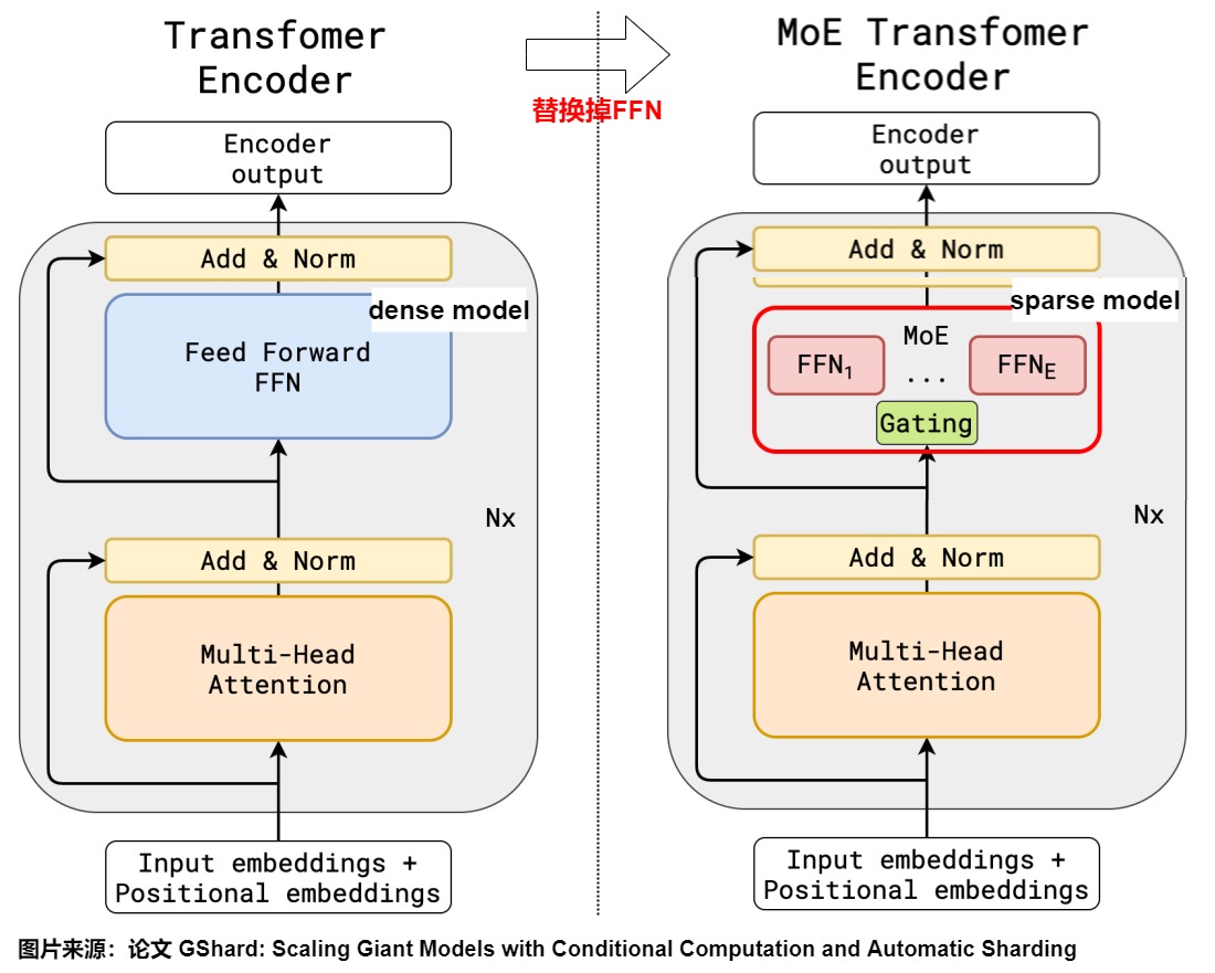
The 2021 paper “GShard: Scaling Giant Models with Conditional Computation and Automatic Sharding” was the first work to extend the ideas of MoE to Transformers. Specifically, GShard replaces the FFN layer every other layer with a MoE structure, where each expert is an FFN (each expert is of the same size). Each token selects a different expert through Gating, defaulting to the top 2.
Because it’s difficult to control the probability of sending tokens to experts, in practice, some experts may receive many tokens while others receive very few. This phenomenon is called uneven expert load. This not only contradicts the design intent of MoE (specialization of expertise) but also affects computational efficiency (e.g., causing uneven load during communication between different GPUs in distributed training). To alleviate the “winner-takes-all” problem and ensure that different experts handle as many tokens as possible, Gshard proposes the following solutions:
- Expert Capacity Load: To ensure load balancing, GShard forces each expert to process fewer tokens than a uniform threshold, which the paper defines as the expert capacity. When both experts selected by a token have exceeded their capacity, the token is considered an overflow token. These tokens are either passed to the next layer via a residual connection or are discarded entirely.
- Local group dispatching: All tokens in a training batch are evenly divided into G groups, with each group containing tokens. All groups are processed independently and in parallel. This ensures that expert capacity is still being implemented and the overall load remains balanced.
- Auxiliary loss: Add an auxiliary loss function to further penalize cases of uneven expert load.
- Random routing: Under the Top-2 gating design, GShard always selects the highest-ranked expert, but the second expert is randomly selected based on their weight ratio. Intuitively, it seems that when the output is a weighted average and the secondary weights are usually small, the contribution of the secondary experts can be ignored.
Gshard also proposed a method for MoE cross-device sharding. When scaling to multiple devices, MoE layers are shared across different devices, while all other layers are copied on each device. In this way, the computation of the entire MoE layer is distributed across multiple devices, with each device handling a portion of the computational task. This architecture is highly efficient for large-scale computation. This also explains why MoE can achieve larger model parameters and lower training costs.
![]()
GShard paved the way for all subsequent MoE research: he demonstrated the value of sparse experts and highlighted the importance of key concepts such as the “capacity factor” for later schemes.
2.1.4 Switch Transformer
The paper “Switch Transformers: Scaling to Trillion Parameter Models with Simple and Efficient Sparsity” replaces the FFN in the Transformer block with a hybrid expert layer with sparse activation, while using a simplified gating mechanism to make training more stable, thus making MoEs a more realistic and practical choice for language modeling applications.
The guiding design principle of Switch Transformer is to maximize the number of parameters in the Transformer model in a simple and computationally efficient manner. Guided by this principle, the paper makes several effective efforts, including simplifying sparse routing, using efficient sparse routing, and enhancing training and fine-tuning techniques. The authors of Switch Transformer found that using only one expert can guarantee model quality. One expert simplifies routing computation and reduces communication; one token corresponds to only one expert, further reducing computation; and the average batch size per expert can be at least halved. Therefore, Switch Transformer’s gating network routes to only one expert at a time, meaning it only selects the top-ranked expert each time, while other models use at least two experts.
![]()
2.2 Detailed Timeline
The following chart provides a timeline overview of several representative MoE models released since 2017. The timeline is primarily constructed based on the model release dates. MoE models above the arrows are open-source, while those below the arrows are proprietary, closed-source models. MoE models from different domains are marked with different colors: green for Natural Language Processing (NLP), yellow for Computer Vision (CV), pink for Multimodal, and cyan for Recommendation Systems (RecSys).
![]()
0x03 Model Structure
MoE includes the following core components:
- Experts. In the MoE architecture, experts are sub-models specifically designed for a particular task. Experts possess expertise in different domains and are responsible for handling different computational tasks or specific input subspaces. Formally, each expert network (usually a linear-ReLU-linear network) is parameterized by parameters , accepts input , and generates output .
- Gating functions (also known as routing functions or routers): Gating functions are responsible for coordinating expert computations, that is, determining which input samples should be processed by which experts, and which experts will be activated and participate in the current computation. Formally, the gating function (usually composed of a linear-ReLU-linear-softmax network) is parameterized by parameters , accepts input and produces output.
- Combining Layer: The combining layer is responsible for integrating the outputs of the expert network to form the final output result. Many resources do not list the combining layer as a separate component.
The entire structure can be represented by the following diagram. The output of the gating network is a sparse n-dimensional vector, where is the weight of the i-th expert given by the gating network, and is the output of the i-th expert. Therefore, for the current input , the output is the weighted sum of all the experts.
![]()
The diagram below illustrates the overall processing flow of MoE, which consists of five steps. Each expert and token is color-coded, and the gating network weights (W) have a representation for each expert (color matching). To determine the route, the router weights perform a dot product on each token embedding (x) to produce a router score (h(x)). These scores are then normalized to 1 (p(x)). G uses the softmax function.
- The gating score is obtained by taking the dot product of the input token’s embedding and the gating network weights. In the context of language modeling, each column here represents a token in the input sequence. Therefore, each token can be routed to a different expert.
- Applying softmax to the gating score normalizes the gating score, yielding a probability. This probability represents the contribution of each expert model to the token, i.e., the probability that each expert is activated given the input context. In other words, this probability indicates the expert’s ability to process the incoming token.
- Use this probability distribution as weights to select the best-matching expert.
- Experts process the input token.
- After expert processing, the output of each router is multiplied by the output of each selected expert, and the results are summed.
![]()
3.1 Gating Function
3.1.1 Condition Calculation
Sparse activation is a key component and one of the advantages of the MoE model. Unlike dense models where all experts or parameters are active in response to the input, sparse activation ensures that only a small subset of experts are activated based on the input data. This approach reduces computational requirements while maintaining performance, as only the most relevant experts are active at any given time.
Essentially, the large MoE models we’re discussing now use conditional computation to enforce sparse activation. Conditional computation explores how to separate computational complexity from computational demands, striking a reasonable trade-off between the two. In this context, it means dynamically turning parts of the neural network on and off. The core of conditional computation in MoE models is learning a computationally inexpensive mapping function that determines which parts of the network—in other words, which experts—can most effectively process a given input. In large models, conditional computation is typically implemented using routing networks or gating networks. It’s crucial for deciding which expert to use, selectively activating certain units in the network based on the input data. In current large language models, this is achieved by conditionally judging each token. When the model inputs a token, the routing network selects the appropriate expert network to compute based on the context and the current token. The direct effect of this selective activation is to speed up the propagation of information within the network, both during training and inference. Through conditional computation or sparsity, large models achieve a suitable balance between increasing model size and reducing computational costs. In fact, the early-exit mechanism, which is common in large model inference, is also a form of conditional computation. It allows decisions to be made at early levels of the network and reduces computation.
Because it uses conditional computation, MoE has a faster inference speed compared to models with the same number of parameters. However, because it uses conditional computation, MoE requires the entire expert system to be fully loaded into memory, thus necessitating a large amount of GPU memory.
3.1.2 Definition
The design and implementation of the gating network is a core component of the sparsely-gated MoE layer. The gating network is responsible for selecting a sparse group of experts for each input token, which will participate in the current computation. The gating function is a network that performs a series of nonlinear transformations, modeling a probability distribution and making appropriate selections based on probabilities. The gating network consists of learned parameters and is pre-trained simultaneously with the rest of the network. A typical gating network is a simple network with a softmax function.
Assuming the input data shape of the attention layer is (batch_size, seq_len, embedding_size), then the size of the gating network is (token_size, expert_num), the input shape of the gating network is (batch_size * seq_len, embedding_size), and the output is (batch_size * seq_len, expert_num), which represents the probability of each token going to each expert. For example:
gates ( batch_size * seq_len = 3, expert_num = 4):
[
    [0.2, 0.4, 0.1, 0.3],  # Token A 被分配到不同专家的概率
    [0.1, 0.6, 0.2, 0.1],  # Token B 被分配到不同专家的概率
    [0.3, 0.1, 0.5, 0.1]   # Token C 被分配到不同专家的概率
]
The gating network learns which expert to send the input to, and the softmax output serves as the final weights for each expert. The gating function’s processing flow is as follows:
- Calculate expert scores. The gating function takes the embedding of a single token as input, performs calculations based on the features of the input data, and then outputs a set of scores. These scores represent the degree of contribution of each expert model to that token, or in other words, indicate how well the experts handle the incoming token.
- Calculate the probability distribution of experts. Taking the following figure as an example, the gating function uses softmax to process the scores, obtaining the probability distribution of each expert’s activation under a given input context. This distribution reflects the magnitude of the correlation between the input data and each expert; the higher the probability, the more important the expert is for the current input prediction task. In the figure below, two experts are selected, and the gating function outputs probabilities of 0.1 and 0.9, indicating that expert 1 contributes 10% to the token, and expert 2 contributes 90%.
- Activating Experts. The gating function takes each token as input and generates a probability distribution over the expert to determine which expert each token is sent to. Based on the probability distribution of the gating output, a subset of experts are selected and activated. In the diagram below, if a top-2 strategy is used for selection, other experts are not selected because their activation probability is less than 0.1. Experts 2 and n-1, with higher activation probabilities, are selected to participate in subsequent calculations. This means that only the parameters of these two experts are used to process the current input data. Assuming expert 2’s output value is 0.4 and expert n-1’s output value is 0.5, the final MoE returns the selected expert’s output multiplied by the gate (selection probability) as 0.49. By simultaneously consulting multiple experts on a given input, the network can effectively weigh and integrate their contributions, thereby improving performance.
![]()
Note: While dynamically training the gating function is standard practice in MoE models, some studies have explored non-trainable token-choice gating mechanisms. The main advantage of this mechanism is that it does not require additional gating network parameters, achieving comprehensive load balancing through a specific gating mechanism. For example, the Hash Layer uses a randomized fixed gating approach, hashing the input tokens without requiring a trained gating network. Other more complex hash functions have also been explored, such as applying k-means clustering to the token embeddings generated by a separately pre-trained Transformer model, or pre-compiling a hash table based on token frequencies in the training data to map token IDs to experts, thus ensuring a more balanced distribution of tokens to experts.
3.1.3 Features
Next, let’s look at the characteristics of gating functions.
First, the gating function determines not only which experts are selected during inference but also which are selected during training. This is because only by allowing each expert to learn different information during training can we determine which experts are most relevant to the given task during inference.
Secondly, the gating function selects an expert at each level. In each level of an LLM with MoE, we find an expert (somewhat specialized). See the diagram below for details.
![]()
In fact, at the most microscopic level, each neuron is an expert, and the activation function acts as a gating function. MoE simply clusters many neurons into one expert.
In addition, both “OpenMoE” and Mixtral have analyzed the gating mechanism, mentioning several characteristics as follows:
- Context-independent specialization. MoE tends to route tokens simply based on token-level semantics, meaning that certain keywords are frequently assigned to the same expert regardless of the context. Because the routing rules are independent of the semantic topic of the text, this means that experts in the MoE model are each good at handling different tokens, but the experts may not actually be experts in any particular domain.
- Early Routing Learning. Routes are established early in pre-training and remain largely unchanged, so tokens are handled by the same experts throughout the training process. This may inspire us to design more efficient routing mechanisms.
- The drop-towards-the-End phenomenon is significant. Tokens at the end of the sequence are more likely to be dropped because experts reach their capacity limits. Specifically, in the MoE model, to ensure load balancing, a capacity limit is typically set for each expert. When an expert reaches its capacity limit, that expert will no longer accept new tokens and will drop them. If we assign experts to tokens in the sequence from front to back, then tokens at the end of the sequence will have a greater probability of being dropped, which is more pronounced in instruction tuning datasets.
- Location locality. Adjacent tokens are often routed to the same expert, indicating that the token’s position in a sentence affects routing and can lead to a “high repetition rate” phenomenon. This can help reduce sudden fluctuations in expert load, but it can also cause experts to be “dominated” by localized data.
Therefore, we need to understand the “local patterns” of the dataset, because once the data distribution changes (for example, from news text to code), its original routing patterns may become invalid. To perform large-scale MoE, we must carefully consider the relationship between data characteristics and expert assignments.
3.1.4 Optimization
Key factors
The overall architecture of the MoE large model is now quite fixed, making routing crucial. Routing algorithms can range from simple (uniform selection or binning based on the tensor’s mean) to complex. Among the many factors that determine the applicability of a particular routing algorithm to the problem, the following are frequently discussed.
- Model accuracy. The MoE model is sensitive to rounding errors; for example, the exponential operation in softmax can introduce rounding errors, leading to training instability. However, simply pruning (i.e., applying a hard threshold to remove large values) the logit output of the gating function can also harm model performance.
- Load balancing. We aim to distribute the number of tokens handled by different experts as evenly as possible. Currently, the simplest solution we know is to select the top k experts based on a softmax probability distribution. However, this approach leads to an unbalanced training load: during training, most tokens are distributed to a few experts, who accumulate a large number of input tokens, while other experts are relatively idle, slowing down training. Meanwhile, many other experts don’t receive sufficient training. Therefore, a better gating function is needed to distribute tokens more evenly among all experts.
- Efficiency is crucial. If gating functions can only be executed serially, load balancing becomes difficult. Assuming we have E experts and N tokens, the computational cost of the gating functions alone is at least . In practice, N and E can be on the order of the letter, and inefficient gating will leave most of the computing resources (experts) idle most of the time. Therefore, we need gating functions that can be implemented efficiently in parallel to utilize numerous devices.
To achieve these goals, researchers have made tireless efforts, and the figure below illustrates the different gating functions used in MoE models. These include (a) a sparse MoE using top-1 gating; (b) a BASE layer; (c) combining domain mapping with stochastic gating; (d) expert selection gating; (e) an attention router; and (f) a soft MoE with expert merging. These functions may be trained through various forms of reinforcement learning and backpropagation to make binary or sparse and continuous, stochastic or deterministic gating decisions.
![]()
Improved Example
Taking the paper “Outrageously Large Neural Networks: The Sparsely-Gated Mixture-of-Experts Layer” as an example, we will see how to upgrade the simple softmax gating function to meet the requirements.
The problem with the softmax function is that it forces all experts to perform calculations on the input, and then performs a weighted sum of the outputs of the gating network. If the number of experts is too large, this leads to an extremely high computational cost. Therefore, we need to find a way to make the output of the gating network for some expert models zero, thus eliminating the need to perform calculations for those experts and saving computational resources.
A standard top-k routing strategy can meet this requirement, selecting the top k experts based on the softmax probability distribution. Specifically, before applying the softmax function to the expert weights, a KeepTopK operation is performed, setting the weights of all experts except the top k to . This ensures that only the top k experts have weights greater than 0 after applying the softmax function. Therefore, this MoE helps us ensure that the computational cost increases non-linearly while scaling the model (because each token only uses the top K experts, not all experts), which is why we call the MoE layer a sparse layer.
A significant drawback of the standard top-k routing strategy is that the gated network may converge to activating only a small number of experts. This is a self-reinforcing problem: if a small subset of experts are disproportionately selected early on, they will be trained much faster, leading to an unbalanced training load. Furthermore, these faster-trained experts will produce more reliable predictions compared to other undertrained experts, and they will continue to be selected more frequently. This unbalanced load means that the other experts will eventually become a real burden.
Noisy Top-K Gating alleviates this problem by adding Gaussian noise to the probability values predicted by each expert. The main reasons for adding noise to the MoE model are as follows:
- Improve the robustness and generalization ability of the model. When the model encounters uncertain or noisy data during the training or inference phase, a more robust model is better able to maintain stable performance.
- Noise adds some randomness, reducing the risk of overfitting.
- Adding noise can achieve load balancing among different experts.
This scheme also adds two trainable regularization terms to expert selection: minimizing the load balancing loss penalizes over-reliance on any single expert, while minimizing the expert diversity loss rewards equal utilization of all experts. The following diagram illustrates this solution.
- The original processing flow is shown in Figure 1 below, where the gating function is softmax. The routing strategy is to multiply the input by the weight matrix and then apply softmax.
- However, this method does not guarantee that the expert’s choices will be sparse. To address this issue, we first perform a linear transformation on the input, and then add a softmax function, resulting in a non-sparse gating function. (See Figure 2 below.)
- However, this is still not enough. Therefore, before performing softmax, we use a topk function to keep only the k largest values and set the rest to . This way, for the non-Topk parts, since the values are negative infinity, they will become 0 after softmax and will not be selected, thus achieving sparsity. Based on this, we add Gaussian noise to the input. This corresponds to number 3 in the diagram below.
![]()
Random routing is another approach to solving this problem. For example, in a top-2 setup, the “best” expert is selected using a standard softmax function, while the second expert is selected semi-randomly (the probability of each expert being selected is proportional to the weight of its connections). Therefore, the second-ranked expert is most likely to be selected, but it is no longer guaranteed that they will be selected.
Another approach to this problem is to adjust based on a threshold for expert capacity. This method sets a threshold that defines the maximum number of tokens any expert can process. Taking the Top-2 expert selection as an example, if any of the top-2 experts has reached its capacity, the next expert (Top 3) is selected to process subsequent tokens. However, this can lead to token overflow, meaning that tokens exceeding the capacity cannot be processed by the designated expert. Additionally, some research has proposed DSelect-k, a smooth top-k gating algorithm whose smoothness is superior to traditional top-k methods.
3.2 Experts
In the MoE architecture, experts refer to pre-trained sub-networks (neural networks or layers) that specialize in handling specific data or tasks. Both experts and gating mechanisms are jointly trained with other network parameters via gradient descent. The term “expert” in MoE is an anthropomorphic representation; in reality, experts are essentially “cross-category sampling” based on some prior human “knowledge” or “strategy.”
3.2.1 Features
Experts possess the following characteristics:
-
Architecture. In practice, each expert in a MoE is generally a feedforward neural network with the same architecture. However, we can also use more complex architectures. We can even create “layered” MoE modules by implementing each expert as another MoE. In some cases, not all FFN layers are replaced by MoEs; for example, the Jamba model has multiple FFN and MoE layers.
-
Parameter subset: The FFN layer is decomposed into multiple experts, each of which is actually a subset of the FFN parameters. The experts are not an average division of the FFN; in fact, we can arbitrarily specify the size of each expert, and each expert can even be larger than the original single FFN layer. This does not change the core idea of MoE: for a token, the computational cost of some experts is less than the computational cost of all experts.
-
Input segmentation: Different experts focus on different topics. In more technical terms, the input space is “regionalized” (or the knowledge space is more finely divided). Suppose an LLM might receive a request that is a “complete knowledge space,” and MoE segments the input data into multiple regions based on task type, and assigns the data in each region to one or more expert models.
-
Focused learning. Each expert model can focus on processing its own input data, learning a specific pattern or feature within the data. Because these experts exist from the beginning, during training, each expert becomes more specialized in certain topics, while others become more knowledgeable in others. For example, in an image classification task, one expert might specialize in identifying textures, while another might identify edges or shapes.
-
Flexible expansion and collaborative operation. In the MoE paradigm, only relevant experts are activated to process a given input. Because only relevant experts are activated, unnecessary computations are reduced (helping us scale the model while ensuring computational costs increase non-linearly), thus accelerating inference and reducing computational costs. Furthermore, MoE can expand the model’s parameter space with reduced computational overhead and without a corresponding increase in computational cost, benefiting from a wealth of expertise. Users don’t need to hire an “omniscient” expert; instead, they can assemble a team with specific domain expertise. This division of labor helps the entire model handle problems more efficiently, as each expert only deals with the data type best suited to them. Additionally, MoE allows the model to adapt more flexibly to different tasks, as different tasks may require combinations of different experts to achieve optimal prediction results.
Let’s look at another example to see what the expert learned.
Current research suggests that experts do not specialize in specific fields such as “psychology” or “biology.” At most, they learn syntactic information at the word level: more specifically, they excel at processing specific tokens within a particular context. The information experts learn is more granular than information across an entire field. Therefore, sometimes calling them “experts” can be misleading.
A good example can be found in the Mixtral 8x7B paper, where the authors measured the distribution of selected experts (token distribution proportions) across different subsets of the Pile validation dataset. The figure below shows the results at layers 0, 15, and 31 (layers 0 and 31 are the first and last layers of the model, respectively). The paper did not observe any obvious patterns when assigning experts based on topic. For example, the expert assignment distributions for ArXiv papers, biology documents, and philosophy documents were very similar across all layers. Only the distribution for mathematics experts differed slightly. This difference is likely a result of the synthetic nature of the dataset and its limited coverage of natural language, particularly evident in the first and last layers, where the hidden states are highly correlated with the input and output embeddings, respectively. This suggests that gating networks do indeed exhibit some structured syntactic behavior.
![]()
Therefore, although experts may not appear to have specialized knowledge, they do seem to be consistently used for certain types of tokens. The figure below shows text examples from different domains (Python code, mathematics, and English), where each token is highlighted with a background color corresponding to its selected expert. The figure shows that words like “self” in Python and “question” in English are frequently passed through the same expert, even when they involve multiple tokens. Similarly, in the code, indentation tokens are always assigned to the same expert, especially in the first and last layers where the hidden states are more relevant to the model’s input and output. We also note from the figure that consecutive tokens are often assigned to the same expert. In fact, the paper’s authors did observe a degree of positional locality in The Pile dataset.
![]()
Therefore, some studies argue that experts improve memory performance rather than reasoning ability. For example, the paper “Mixture of Parrots: Experts improve memorization more than reasoning” investigated the theoretical limitations of the Mixture-of-Experts (MoE) architecture in terms of performance and reasoning, exploring its performance differences from standard memory-intensive Transformers in terms of memory and reasoning. The study found that as the number of experts increases, the MoE model improves its performance on memory tasks, but reaches saturation on reasoning tasks. The paper also empirically demonstrated the superiority of MoE on specific memory-intensive tasks.
Furthermore, the MoE model actually provides a fine-grained way to study and understand the internal workings of a model. By observing which experts are activated and how they change over time, researchers can gain deeper insights into how the model learns and generalizes knowledge, and how it handles different input features.
3.2.2 Types
Experts typically fall into the following network types:
- Feed-Forward Networks (MoEs): Because FFN layers are sparser than self-attention layers and exhibit more domain specificity, most MoEs are currently replacements for FNNs. For example, researchers have found that most inputs activate only a small number of neurons in the FFN, highlighting the inherent sparsity of the FFN. For the same input, the FFN layer activates only 20% of the experts, while the self-attention layer activates 80%. Emergent modularity in pre-trained Transformers also reveals a significant correlation between neuron activation and task-specificity, supporting the view that the MoE structure reflects the modularity of pre-trained Transformers. Furthermore, the choice is also evident from the perspective of parameter count, as the computational cost of FFNs increases dramatically with model size. For example, in the PaLM model with 540 billion parameters, approximately 90% of the parameters are distributed in the FFN layer.
- Attention: While MoE research primarily focuses on the FFN layer of the Transformer architecture, some researchers have proposed Mixture of Attention Heads (MoA), combining multi-head attention layers with MoE to improve performance and reduce computational cost. MoA uses two sets of experts (query projection and output projection), selecting the same experts through a common gating network. To reduce computational complexity, MoA shares and projection weights among all attention experts. Experts differ only in their respective query () and output projection weights (), thus achieving pre-computation sharing of key () and value () sequences.
- Other types. Some researchers have also explored using convolutional neural networks (CNNs) as experts, and there have been efforts to combine parameter efficient fine-tuning (PEFT) techniques with MoE, such as using low-rank adaptation (LoRA) as an expert.
![]()
3.2.3 Location
Next, let’s look at how experts are embedded in the Transformer architecture. The following diagram provides some examples.
- (a) demonstrates the integration of MoE with the Key and Value modules in the attention mechanism.
- (b) indicates the application of MoE in FFN.
- (c) refers to the integration of MoE at the Transformer block level, in which two different sets of experts are applied to the attention and FFN layers, with experts assigned to each layer and regulated through their respective gating mechanisms.
- (d) shows the integration of MoE at each layer, where each Transformer layer is treated as a unified entity and gating mechanisms coordinate the interactions between experts.
![]()
3.3 Classification
In our previous studies, we gained a general understanding that there are different types of MoEs. Here, we’ll examine how to classify MoEs from the most fundamental perspective (gating functions). Gating functions are the core of the MoE architecture; they are responsible for coordinating the participation of expert networks and integrating their outputs. Based on different input processing methods, gating mechanisms can be divided into three categories: sparse, dense, and soft. Sparse gating activates only some experts, dense gating activates all experts, and soft gating includes total differential methods, such as input token merging and expert merging. The characteristics of the three types of gating functions are as follows:
- Sparse gating: Activating only a subset of experts, including top-k gating strategies based on token selection, and using auxiliary loss functions to promote uniform token distribution among experts.
- Dense Gating: Activates all experts and performs exceptionally well in LoRA-MoE fine-tuning because it can effectively integrate multiple LoRAs into a variety of downstream tasks.
- Soft gating: Achieves full differentiability through tokens or expert merging, avoiding the problem of discrete expert selection, such as SMEAR, Lory, and Omni-SMoLA.
Based on the design of the gating function, MoE layers can be roughly divided into the following two categories: dense MoE and sparse MoE.
- Dense MoEs can fully utilize all parameters, capturing potentially complex patterns and relationships, thus typically achieving higher prediction accuracy, but with higher computational cost. Therefore, this method was widely adopted in early research, and recent studies (EvoMoE, MoLE, LoRAMoE, and DSMoE) have re-examined the application of dense MoEs. While sparse activation of experts has advantages in computational efficiency, it often leads to performance loss when the total number of parameters is the same. In LoRA-MoE fine-tuning, dense activation performs well due to the lower computational cost of LoRA experts. This method can effectively integrate multiple LoRAs into various downstream tasks, maintaining both the generative capability of the original pre-trained model and the uniqueness of each task-specific LoRA.
- A dense MoE layer activates all expert networks in each iteration.
- A sparse MoE layer activates only a selected subset of experts in each forward pass. Instead of aggregating the outputs of all experts, sparse MoEs achieve sparsity by computing only a weighted sum of the outputs of the top k experts. Sparse activation is essentially a trade-off between computational requirements and model performance.
The figure below illustrates the characteristics of two MoEs. The right side is a schematic diagram, and the left side shows the gating function and the load function.
![]()
3.3.1 Dense vs. Sparse
We use examples to compare dense and sparse MoE.
Take the division of labor in humans as an example. Dense labor is similar to the production model of the handicraft era. In this model, each worker (i.e., neuron) needs to participate in processing all types of tasks, just as a craftsman in the handicraft era needed to be proficient in every aspect of product making and master all production skills. Although this method is intuitive and easy to implement, it is often inefficient and difficult to scale when faced with complex and ever-changing tasks. Sparse labor, on the other hand, is the division of labor model after the Industrial Revolution: each position (expert) only needs to complete a portion of the production tasks. This division of labor greatly improved production efficiency, promoted the process of industrialization, and ushered in the era of large-scale machine industry.
![]()
3.3.2 Soft Gating
The paper “A Survey on Mixture of Experts” introduces the soft-gated type to highlight its ability to alleviate computational demands by merging input tokens or experts through gated weighting. Sparse MoEs typically require heuristic auxiliary losses to ensure a balance of expert participation in order to assign appropriate experts to each input token. These issues become even more pronounced in scenarios involving out-of-distribution data. Similar to dense MoEs, soft MoE methods avoid the problems inherent in discrete expert selection by leveraging all experts to process each input while maintaining full differentiability.
- Token Merging: Soft MoE abandons traditional sparse and discrete gating mechanisms, employing a soft allocation strategy to merge tokens. This method calculates a weighted average of all tokens, with weights depending on the relationship between the token and the expert, and then processes each weighted average result with the corresponding expert. However, token merging makes it difficult to apply to autoregressive decoders because future tokens used for weighted averaging cannot be obtained during inference.
- Expert Merging: The SMEAR framework avoids discrete gating by merging all expert parameters through a weighted average. The authors of SMEAR argue that traditional sparse MoE models struggle to compete with dense models of comparable parameter counts or models using non-learning heuristic gating functions, possibly due to gradient estimation biases in the training modules of non-differentiable, discretely gating decision-making systems. SMEAR processes input tokens through a single merged expert, without significantly increasing computational cost, while still supporting standard gradient training.
3.4 Comparison
The paper “A Uniffed View for Attention and MoE” compares the attention mechanism with MoE. The role of the attention structure is essentially to aggregate information from different tokens using a weighted sum. MoE, on the other hand, learns a router through linear projection and aggregates information from different experts based on that router. Essentially, the router’s output is processed through top-k+softmax to learn a weighted sum, ultimately aggregating information from different tokens.
Similarities between the two:
- Both use softmax to normalize the weights, essentially aiming to learn stable values.
- Essentially, they are all weighted sums of new features.
- They are all dynamic weights, which adaptively aggregate information based on the input.
The difference between the two is that
- Attention aggregates information from different tokens, while MoE aggregates information from different Experts.
- Attention uses all tokens (Softmax results in a positive number, so all tokens are used); MoE is a sparse selection that only selects a subset of the results.
- Both Attention and MoE learn weights to aggregate information, which can be summarized as shown in Figure 3 below, where f is the weight and g is the learned new feature. See the figure below for details.
![]()
This also offers insights from a computer architecture perspective. Attention mechanisms (including FFN) are similar to storing all context in memory. MoE can be understood as a page table system, where the page table corresponding to an expert is only put into memory when needed.
0x04 Calculation Process
4.1 Algorithm
The following diagram shows the pseudocode for the top-k gated function algorithm. The specific process is as follows.
- Given input x, use a gating function to compute the score
score = G(x). - Select the indices corresponding to the top k scores.
- Traverse the index and use the expert corresponding to the index to perform calculations to obtain the reasoning result.
- The expert-calculated results are corrected using scores as weights.
- The results from these k experts are combined to form the final inference.
![]()
4.2 Process
The entire calculation process of MoE is shown in the figure below:
- Routing, also known as “experts selection” or sparse activation, is essentially the use of gating functions and is a core concept of MoE. Routing is a multi-classification discrimination process for inputs, aiming to determine the most suitable expert model to handle the input. In language model applications, when the input token passes through the MoE layer, the token is multiplied by the Router’s weight matrix to obtain an Expert Indices (decision matrix) and a probability tensor, namely the index and probability.
- Expert indices is an expert-to-token mapping used to indicate which expert each token is assigned to. That is, the i-th value in the tensor represents the expert to whom this token should be assigned.
- The Probabilities tensor represents the probability of the allocated confidence level, where the i-th value represents the weight of the expert for the final result of the token.
- Permutation. Tokens are allocated to the corresponding experts based on routing decisions (expert-to-token mapping). Tokens may be discarded during this process depending on the expert’s capacity.
- Computation. Experts perform computations based on permutation-reordered tokens. This approach achieves computational efficiency by focusing each expert on a specific task. This allows the model to personalize its processing for different types of input data, improving overall efficiency and performance. Each expert network processes its assigned tokens in parallel, computing the output. This step involves block sparse matrix multiplication, where the input matrix 𝑥″ is multiplied by the weight matrix of the expert network. Let 𝑊 be the weight matrix of the expert network, then the output of the expert network can be represented as: 𝑦 = 𝑥″ × 𝑊, where 𝑦 is the sum of the outputs of all expert networks.
- Un-Permutation. This involves collecting the experts’ computational results. It’s the inverse of Permutation, aiming to combine the processed tokens collected from various experts into a complete sequence that maintains the original token order. Specifically, it rearranges the outputs of each expert network according to the original token order. Let 𝑦 be the sum of all expert network outputs; the un-permutation operation can be represented as: 𝑦′ = scatter(𝑦, 𝑖𝑛𝑑𝑖𝑐𝑒𝑠), where 𝑦′ is the final model output. The scatter operation rearranges the outputs in 𝑦 according to the indices in 𝑖𝑛𝑑𝑖𝑐𝑒𝑠 to match the original token order. The results are then scaled (weighted summation) using the distributed confidence probabilities generated in the Routing step to obtain the final model output, which is then further processed downstream.
![]()
Because permutation is relatively complex, we will analyze it in detail below.
4.3 Permutation
The main function of permutation is:
- Token distribution. Permutation constructs a local temporary matrix based on Expert Indices, rearranging the input tokens according to the routing results. This allows tokens belonging to each expert to be grouped together before being sent to the corresponding expert. This enables each expert network to process its assigned tokens in parallel, ensuring the model fully utilizes the parallel computing power of the GPU. For example, in the diagram above, “the” and “jumped” should be assigned to expert 1, so they are grouped together. “quick” and “fox” should both be sent to expert 2, so they are also grouped together.
- Maintaining the order of tokens and experts is crucial. Since a batch contains many tokens, sending them to different experts for computation will inevitably shuffle the expert outputs. Therefore, a method is needed to track the order, permuting the tokens back to their correct positions before inputting them into the next layer of the network. Through the constructed matrix, permutation can maintain this order during computation.
- Load balancing. Permutation enables the rational distribution of input data among different experts to balance their computational load. Different input samples may have different computational resource requirements for different experts. By permuting the input samples, each expert can receive the samples that need to be processed relatively evenly, avoiding situations where some experts are overworked while others are idle.
- Increase diversity. Permutation can increase the diversity of how the model processes the input data. This is because different permutation orders may lead to different expert combinations processing the data, thereby uncovering different features of the data.
From an algebraic perspective, MoE computation is essentially performing a permutation group operation on the tokens: . P (the permutation operation) is a sparse matrix that performs token position permutations, which also forms an algebraic permutation group structure. needs to restore the tokens to their original order, ensuring they are output to the next layer. The fundamental problem in MoE implementation is how to parallelize the sparse matrix multiplication constructed based on the permutation matrix.
4.4 Implementation
4.4.1 Mistral Inference
We’ll start by learning from https://github.com/mistralai/mistral-src, as this code is relatively simple and easy to understand. Here, gate is the gating function, configured as follows: gate=nn.Linear(dim, moe.num_experts, bias=False).
Suppose we define 4 experts, and the routing selects the first 2 experts, i.e., num_experts=4, num_experts_per_tok=2, and the word embedding size is 32. MoE receives the output of the attention layer as input X, which projects the input from the shape [2, 4, 32] of (batch_size, sequence_length, input_dim) to the shape [2, 4, 4] corresponding to (batch_size, sequence_length, num_experts), where num_experts is expert=4. Then, the tensor is transformed to [2, 4, 2] using torch.topk. The selected_experts returned by torch.topk can be understood as the indexes of the two experts selected for each token.
![]()
The specific code is as follows.
import dataclasses
from typing import List

import torch
import torch.nn.functional as F
from simple_parsing.helpers import Serializable
from torch import nn


@dataclasses.dataclass
class MoeArgs(Serializable):
    num_experts: int # 专家数量
    num_experts_per_tok: int # 每一个token被分配给几个专家

# gate=nn.Linear(dim, moe.num_experts, bias=False)
class MoeLayer(nn.Module):
    def __init__(self, experts: List[nn.Module], gate: nn.Module, moe_args: MoeArgs):
        super().__init__()
        assert len(experts) > 0
        self.experts = nn.ModuleList(experts)
        self.gate = gate
        self.args = moe_args

    def forward(self, inputs: torch.Tensor) -> torch.Tensor:
        gate_logits = self.gate(inputs) # 通过门控网络获得各个专家的logits
        # 取出topk(k=2)专家的权重以及专家索引
        weights, selected_experts = torch.topk(gate_logits, self.args.num_experts_per_tok)
        #使用softmax来归一化权重
        weights = F.softmax(weights, dim=1, dtype=torch.float).to(inputs.dtype)
        # 创建形状和x一致,初始值为0的矩阵,用来存储每个expert的输出
        results = torch.zeros_like(inputs)
        for i, expert in enumerate(self.experts): #遍历每一个专家
            # selected_experts == i 得到的是一个矩阵,行为token的idx,列为专家的idx
            batch_idx, nth_expert = torch.where(selected_experts == i)
            # 每一个token的结果都是由2个专家的结果进行加权求和得到的
            # 利用None来增加维度,新增维度大小为1,有几个None就会增加几个维度。
            results[batch_idx] += weights[batch_idx, nth_expert, None] * expert(inputs[batch_idx])
        return results
The code below shows that the gated network is an instance of nn.Linear, while the expert network is an instance of FeedForward.
class FeedForward(nn.Module):
    def __init__(self, args: TransformerArgs):
        super().__init__()
        self.w1 = nn.Linear(args.dim, args.hidden_dim, bias=False)
        self.w2 = nn.Linear(args.hidden_dim, args.dim, bias=False)
        self.w3 = nn.Linear(args.dim, args.hidden_dim, bias=False)

    def forward(self, x) -> torch.Tensor:
        return self.w2(nn.functional.silu(self.w1(x)) * self.w3(x))

class TransformerBlock(nn.Module):
    def __init__(self, args: TransformerArgs):
        super().__init__()
        self.n_heads = args.n_heads
        self.dim = args.dim
        self.attention = Attention(args)
        self.feed_forward = MoeLayer(
            experts=[FeedForward(args=args) for _ in range(args.moe.num_experts)],
            gate=nn.Linear(args.dim, args.moe.num_experts, bias=False),
            moe_args=args.moe,
        )
        self.attention_norm = RMSNorm(args.dim, eps=args.norm_eps)
        self.ffn_norm = RMSNorm(args.dim, eps=args.norm_eps)
        self.args = args

    def forward(
        self,
        x: torch.Tensor,
        freqs_cis: torch.Tensor,
        positions: torch.Tensor,
        mask: Optional[torch.Tensor],
    ) -> torch.Tensor:
        r = self.attention.forward(self.attention_norm(x), freqs_cis, positions, mask)
        h = x + r
        r = self.feed_forward.forward(self.ffn_norm(h))
        out = h + r
        return out
4.4.2 Mixtral 8x7B
We are learning using Mixtral 8x7B, which has a more complex implementation. Code source: transformers / src / transformers / models / mixtral
Below is the code for the MoE layer. The mask matrix in the code is the key focus here. Because in MoE, not all inputs need to pass through all experts. Usually, only a subset of inputs are processed by specific experts. Therefore, a mask matrix is used to determine which input tokens interact with which experts. There are several possibilities for using the mask matrix; for example, for an input batch, the mask matrix can be:
- Specify whether each input sample is processed by expert 1, expert 2, expert 3, or a combination of several experts.
- Alternatively, an element in the mask matrix can be set to 1 to indicate a connection between the corresponding token and the expert (i.e., the expert will process the input), while 0 indicates no connection.
- It can also be used in conjunction with expert capacity for filling.
Furthermore, during training, the mask matrix is used to correctly compute and update the expert parameters. Since only experts connected to the input should contribute to the loss of that input, the mask matrix allows for accurate calculation of the gradient for each expert, thus correctly updating their parameters and avoiding erroneous updates to the parameters of experts who did not process a particular input.
class MixtralSparseMoeBlock(nn.Module):
    """
    This implementation is
    strictly equivalent to standard MoE with full capacity (no
    dropped tokens). It's faster since it formulates MoE operations
    in terms of block-sparse operations to accomodate imbalanced
    assignments of tokens to experts, whereas standard MoE either
    (1) drop tokens at the cost of reduced performance or (2) set
    capacity factor to number of experts and thus waste computation
    and memory on padding.
    """

    def __init__(self, config):
        # 初始化了MoE层中使用到的各个部分参数
        super().__init__()
        self.hidden_dim = config.hidden_size
        self.ffn_dim = config.intermediate_size
        # 设置专家数量
        self.num_experts = config.num_local_experts
        # 设置要选择的topk专家数量
        self.top_k = config.num_experts_per_tok

        # gating
        # 初始化线性层作为门控机制
        self.gate = nn.Linear(self.hidden_dim, self.num_experts, bias=False)

        # 创建专家网络的列表,每个专家是一个 MixtralBlockSparseTop2MLP 实例
        self.experts = nn.ModuleList([MixtralBlockSparseTop2MLP(config) for _ in range(self.num_experts)])

        # Jitter parameters
        self.jitter_noise = config.router_jitter_noise

    def forward(self, hidden_states: torch.Tensor) -> torch.Tensor:
        """ """
        # 将注意力模块的输出隐状态hidden_states作为专家模块的输入。
        batch_size, sequence_length, hidden_dim = hidden_states.shape
        if self.training and self.jitter_noise > 0:
            hidden_states *= torch.empty_like(hidden_states).uniform_(1.0 - self.jitter_noise, 1.0 + self.jitter_noise)
        # 原有hidden_states形状为[batch_size, sequence_length, hidden_dim],为方便计算,将batch_size和sequence_length合并,重构为一个形状为(batch * sequence_length, n_experts)的二维张量。而且,后续计算不是样本维度,而是token维度,这样更清晰
        hidden_states = hidden_states.view(-1, hidden_dim)
        # 将hidden_states导入门控网络中,输出一个路由逻辑用于后续专家分配
        # 计算每个专家的分数,router_logits的形状为[batch_size * sequence_length, n_experts]
        router_logits = self.gate(hidden_states)
		# 计算专家经过softmax之后的概率,最后选取top k个专家用于输出(在dim=1进行softmax处理,即对应路由逻辑中的n_experts以及hidden_states中的hidden_dim)
        routing_weights = F.softmax(router_logits, dim=1, dtype=torch.float)
        # 通过门控函数获得分数最高的 top_k 和门控权重和专家索引
        # selected_experts和router_weight的形状都是 (b * s, top_k)
        routing_weights, selected_experts = torch.topk(routing_weights, self.top_k, dim=-1)
        # 最后对专家权重进行归一化,确保权重之和为1,并且将权重的类别和输入统一
        routing_weights /= routing_weights.sum(dim=-1, keepdim=True)
        # we cast back to the input dtype
        routing_weights = routing_weights.to(hidden_states.dtype)

        # 将token导入对应的专家网络中进行前向传播得到输出
        final_hidden_states = torch.zeros( # 初始化全零矩阵,后续叠加为最终结果
            (batch_size * sequence_length, hidden_dim), dtype=hidden_states.dtype, device=hidden_states.device
        )

        # One hot encode the selected experts to create an expert mask
        # this will be used to easily index which expert is going to be sollicitated
        # 生成专家掩码,具体是根据专家网络的总数量构建一个one_hot编码,根据输入token所分配的专家网络,将one_hot编码中对应的专家网络索引由0变为1,据此来索引给定的专家网络,掩码原始形状是是 (b * s, top_k, expert_number),permute之后形状是(expert_number, top_k, b * s)
        expert_mask = torch.nn.functional.one_hot(selected_experts, num_classes=self.num_experts).permute(2, 1, 0)

        # Loop over all available experts in the model and perform the computation on each expert
        # 在循环中依次通过各个专家网络处理每个输入token
        for expert_idx in range(self.num_experts):
            #依次取出专家网络
            expert_layer = self.experts[expert_idx]
            # expert_mask[expert_idx] shape 是 (top_k, b * s)
            # idx 和 top_x 都是一维张量
            # idx 的值是 0 或 1, 表示这个token认为当前专家是 top1 还是 top2
            # top_x 的值是 token 在展平之后的 batch*seq_len 个token中的位置索引
            idx, top_x = torch.where(expert_mask[expert_idx])

            # Index the correct hidden states and compute the expert hidden state for
            # the current expert. We need to make sure to multiply the output hidden
            # states by `routing_weights` on the corresponding tokens (top-1 and top-2)
            # 找出当前专家网络应该处理的,对应第top_x个token所对应的隐向量hidden_states
            # hidden_states 的形状是 (b * s, hidden_dim)
            current_state = hidden_states[None, top_x].reshape(-1, hidden_dim)
            # 将hidden_states传入到专家网络当中进行处理
            # router_weights的形状是 (b * s, top_k)
            current_hidden_states = expert_layer(current_state) * routing_weights[top_x, idx, None]

            # However `index_add_` only support torch tensors for indexing so we'll use
            # the `top_x` tensor here.
            # 将输出存入之前定义的张量当中
            final_hidden_states.index_add_(0, top_x, current_hidden_states.to(hidden_states.dtype))

        # 将计算完成的输出形状还原为之前的形状 (b * s, expert_number)
        final_hidden_states = final_hidden_states.reshape(batch_size, sequence_length, hidden_dim)
        return final_hidden_states, router_logits
The expert network code is as follows. Mixtral 8x7B uses a three-layer MLP as the expert network in MoE. All three fully connected layers in the MLP participate in forward propagation, and the final output is obtained by weighting the outputs of the fully connected layers and the expert network. The difference between this and the Mixtral of Experts code is that the activation function is represented by a configuration item, which is more flexible, such as hidden_act="silu".
class MixtralBlockSparseTop2MLP(nn.Module):
    def __init__(self, config: MixtralConfig):
        super().__init__()
        self.ffn_dim = config.intermediate_size
        self.hidden_dim = config.hidden_size

        self.w1 = nn.Linear(self.hidden_dim, self.ffn_dim, bias=False)
        self.w2 = nn.Linear(self.ffn_dim, self.hidden_dim, bias=False)
        self.w3 = nn.Linear(self.hidden_dim, self.ffn_dim, bias=False)

        self.act_fn = ACT2FN[config.hidden_act]

    def forward(self, hidden_states):
        current_hidden_states = self.act_fn(self.w1(hidden_states)) * self.w3(hidden_states)
        current_hidden_states = self.w2(current_hidden_states)
        return current_hidden_states
4.5 Number of Parameters
What makes MoE interesting is largely its computational requirements. Because only a subset of experts is used within a given timeframe, we have access to more parameters than we are currently using. But how do we calculate the number of parameters in MoE and its memory footprint?
There are currently two methods for “attribution” of large MoE models, each with its own advantages and disadvantages.
- Names like “8x22B” indicate that the model has 8 experts, each with 22B parameters. The advantage is that it clearly shows the number of experts and the model’s size; the disadvantage is that it can easily mislead people into thinking the model only has 8x22B parameters.
- Names like “57BA14B” indicate a total parameter size of 57 bytes, with 14 bytes activated during each inference. However, it’s unclear how many experts are involved or the size of each expert.
Therefore, some researchers suggest labeling the MoE model as follows: total number of parameters - number of activated parameters - number of ordinary experts - number of activated experts - number of shared experts, which we will explain below.
- Total number of parameters. In reality, the expert is only part of the model; there are also attention layers, embedding layers, LM Head, gating networks, and other modules. The total number of parameters is often referred to as the sparse parameter count, which can be understood as a measure of model capacity and a reference value for how much VRAM is needed during inference, because all the model’s parameters must be loaded into VRAM/RAM.
- Activated parameters. This refers to the actual number of parameters used to process a single token. Since this token only goes through some expert blocks but not others, meaning we only use a subset of experts during inference, the number of activated parameters is relatively small. This metric can be understood as a measure of the computational cost during model inference. In other words, the MoE model requires more VRAM to load the entire model (including all experts), but because only a subset of experts are used during inference, MoE activates fewer parameters and runs faster during inference.
- The number of ordinary experts minus the number of activated experts minus the number of shared experts. This varies depending on the implementation of different MoEs, as some MoEs only have experts and no shared experts. If each Transformer layer has 64 ordinary experts and one shared expert, with 8 activated experts, then during inference, 8 experts will be selected from the 64 ordinary experts for activation. The main parameters loaded during inference at this layer are: number of activated experts * expert size + number of shared experts * expert size + attention layer size + gating function size.
In addition, even if each input uses only a subset of the parameters, the complete parameter set of all experts usually needs to be loaded into memory, which can increase the overall memory usage during the inference process.
4.6 Computational complexity
During the actual computation of inference, each token is gated through a network to select one or more Experts, and then a computation similar to FFN is performed. We can refer to the formula for the computational complexity of MoE given in the paper “Scaling Laws for Fine-Grained Mixture of Experts,” with specific metrics as follows:
- G (Granularity): Granularity, which is how many fine-grained experts a complete FFN is divided into. For example, an FFN can be divided into 8 small experts, and the number of parameters of each expert is 1/8 of the original FFN.
- E (Expansion rate): This refers to how many times the number of parameters from all experts expands to the number of parameters in a single standard FFN. For example, if
G=8and there are a total of 64 fine-grained experts, thenE=64/8=8, which is equivalent to having 8 FFNs of the same standard size. This metric can be understood as the proportion of the total number of MoE parameters to its activation parameters. - D: Number of tokens.
- cf: Represents the ratio of computational cost (excluding Router) to parameter cost, set to 6 in the paper. For each token, the FLOPs of an active parameter in the linear layer are 6. The operation decomposition is as follows:
- During forward propagation, two operations (single multiplication and single addition) are used to compute the matrix multiplication of the input and the linear projection.
- During backpropagation, two operations are used to compute the gradient of the input.
- During backpropagation, two operations are used to compute the gradient of the linear layer weights.
- cr: Represents the ratio of the computational cost to the number of parameters of the router. For simpler routers, it is usually between 6 and 20. A detailed breakdown is as follows:
- During the forward propagation, two operations are used to compute expert logits based on the input and the “routing linear layer”.
- During backpropagation, two operations are used to compute the gradient of the “routing linear layer” with respect to the input.
- During backpropagation, two operations are used to compute the gradient of the “routing linear layer” with respect to the linear layer.
- During the forward propagation, two operations are used to route the input token to the selected expert.
- During the forward propagation, two operations are used to route the expert’s output back to the selected token and multiply these outputs by the routing score.
- During backpropagation, two operations are used to route the gradient from the output token back to the expert.
- During backpropagation, two operations are used to route the gradient from the expert to the input token.
Similar to the FLOP calculation in cf, the FLOP in cr is also in pairs because each multiplication is followed by an addition (used to accumulate the output or gradient).
![]()
Since the computational cost of the Router is usually very small, it can often be ignored. If we do not consider the computational cost introduced by the Router, since each Expert is actually the same as the FFN of the non-MoE model, we can also deduce in the same way that the computational cost of each Token during training is still C=6ND, except that N here is no longer the number of parameters of the entire model, but the number of parameters activated by each Token.
0x05 Parallel Computing
The parallel processing of MOE Transformer layers is generally as follows:
- The non-expert component (attention mechanism) employs tensor parallelism and data parallelism;
- The expert component employs both expert parallelism and tensor parallelism.
5.1 Communication Requirements
Let’s first look at the communication requirements in MoE computation.
5.1.1 Single token
The following diagram illustrates the computation process of a Transformer layer in an MOE structure, where:
w1/w2represent the inputs to the self-attention module;a1/a2represent the outputs of the self-attention module and the inputs of the FFN;f1/f2represents the output of FFN;
The process consists of five steps: 1) organizing, 2) sending, 3) calculating, 4) returning via the original path, and 5) weighted summation. Steps 2 and 4 require communication.
![]()
5.1.2 Multiple tokens
The above operations are performed on each token individually, so it seems simple. However, it’s important to understand that we typically process all tokens in a batch simultaneously, so the above operations, whether for transmission or computation, require modifications to the matrix. Furthermore, we don’t know exactly which cards the k experts selected for a single token are on. Therefore, the complexity of MoE implementation lies in the sorting and transmission.
The actual communication operation is shown in the diagram below. In expert parallel mode, All-to-All communication operations are introduced before and after the expert layer. The first All-to-All operation sends the tokens on each Worker to the expert’s GPU according to the Router, also called All-to-All Dispatch; the second All-to-All operation rearranges the tokens calculated by the expert in the original way, also called All-to-All Combine. It can be seen that there are two communication requirements here:
- Send the token to the expert (for number 1 in the diagram below). The token needs to be sent to the corresponding GPU according to the expert-to-token mapping sequence.
- Collect k calculation results (for symbol 2 in the diagram below). The tokens need to be restored to ensure they are output to the next layer in the original token order.
![]()
The above mentioned two concepts: expert parallelism and all-to-all communication. Let’s analyze them separately.
5.2 Parallel Expert Implementation
When faced with large and complex models, how to efficiently utilize computing resources and improve training speed has always been a focus of researchers. Traditional approaches typically accelerate computation through data parallelism and model parallelism, but these methods are not well-suited for MoE models due to their sparsity and dynamic nature. Therefore, researchers have proposed expert parallelism, which achieves parallel gating and expert computation by distributing partitioned local tokens and limiting the load balancing of expert capacity. Currently, expert parallelism has become a fundamental strategy for promoting the efficient scaling of MoE models.
5.2.1 Definition
Expert parallelism is essentially a model parallelism approach, but it can also be seen as an extension of data parallelism. The idea behind expert parallelism is to distribute different experts in the MoE layer to different computing devices. Each device is responsible for storing and computing a portion of the experts, while all non-expert layers are copied between devices. The expert parallelism process includes the following sequential operations: gated routing, input encoding, all-to-all dispatch, expert computation, all-to-all combine, and output decoding.
- Each EP rank contains only a subset of experts, and the tokens (i.e., the hidden states corresponding to the tokens) on each EP rank are distributed to experts on other EP rank based on the results of gating routing.
- Similar to data-parallel solutions, the input to each card is a complete task, which needs to be masked and decomposed into different subtasks at both the batch and sequence dimensions of each card task. Therefore, expert parallelism uses input encoding to aggregate the input tokens sent to the same expert into a contiguous memory space. This space is determined by the gated routing token-expert mapping, and this operation is called permutation.
- Subsequently, each device will use All-to-All dispatch to send the input token (its respective task) to the device where the corresponding expert is located, according to the routing rules of the MoE model.
- After local computation by experts, the reverse process (All-to-All combine and output decoding) restores the original data layout based on the gating index and returns the result to the original device, thus restoring the complete task on each card.
Because the experts are carefully distributed across various nodes, but each node has a different task. Each node possesses unique expert resources, and the data is cleverly partitioned to ensure a balanced distribution across all nodes, resulting in more efficient use of computing resources.
Note: To achieve the optimal utilization and throughput required by computing devices, the input size of General Matrix Multiplication (GEMM) needs to be large enough.
![]()
5.2.2 History
Industry pioneer
The paper “Outrageously Large Neural Networks: The Sparsely-Gated Mixture-of-Experts Layer” was the first to use an expert parallelism scheme, which it described as “Mixing Data Parallelism and Model Parallelism”.
The paper encounters the following problems. On modern CPUs and GPUs, large batch sizes are needed to improve computational efficiency, thus amortizing the overhead of parameter loading and updates. If the gating network selects k experts from n experts for each example, then assuming a batch contains b samples, each expert receives samples . If the number of experts increases, this leads to very low efficiency in the native MoE implementation; that is, the average number of samples per expert is much smaller than b, which is detrimental to model scaling. The solution to this batch shrinking problem is to make the original batch as large as possible. However, the batch size is often limited by the memory required to store forward and directional propagation activations.
To address this issue, this paper employs the following technique to increase the batch size. The paper runs different batches synchronously, allowing them to be combined for use by the MoE. The other regular layers and gated networks in the model are distributed as in traditional data-parallel schemes, but each expert retains only a shared copy. Each expert in the MoE layer receives a combination of relevant samples from all data-parallel input batches. The same set of devices can act as data-parallel replicas (other regular layers and gated networks) or as model-parallel shards (each device carrying a subset of experts from the expert set). If the model is distributed across d devices, each processing a batch of data of size b, then each expert receives a batch of approximately samples . Therefore, we achieve a d-fold increase in the expert batch size.
![]()
Gshard
Gshard refined the method of MoE’s cross-device sharding. When scaling to multiple devices, MoE layers are shared across different devices, while all other layers are replicated on each device. In this way, the computation of the entire MoE layer is distributed across multiple devices, with each device responsible for handling a portion of the computational tasks. This architecture is highly effective for large-scale computing. Gshard truly demonstrated that training models with hundreds of billions or even trillions of parameters is achievable by intelligently splitting layers and tokens and distributing them evenly among experts.
![]()
Switch Transformers
Switch Transformers is likely the first paper to explicitly propose the concept of expert parallelism. The authors attempted to balance the relationship between the FLOPs per token and the model parameters. Because with the native MoE implementation, increasing the number of experts increases the number of parameters without changing the FLOPs per token. To increase FLOPs, we must also increase (which increases the number of parameters but slows down the process). This necessitates a series of trade-offs: increasing exhausts the memory of each core, requiring an increase in m. However, since the number of cores is fixed at N, and , we must reduce n, which forces the use of a smaller batch size (to maintain a constant number of tokens per core). Therefore, the paper employs expert parallelism.
Note: Assume N is the total number of cores, n is the data parallelism, m is the model parallelism, E is the number of experts, and C is the expert capacity.
summary
Expert parallelism first distributes and saves experts to different devices, then combines input tokens that follow the same data path to form token groups (these tokens select the same expert), and then allows different token groups (different data paths) to perform parallel computation simultaneously.
In non-expert parallel schemes, the more experts there are, the smaller the batch size each activated expert receives. Expert parallelism, however, ensures that the batch size for each expert is proportional to the number of experts. As long as the batch size (d*b, d devices, each processing a batch of b data) increases with the number of experts, the number of samples received by each expert remains constant. This also keeps the memory and bandwidth requirements essentially constant, reducing data access overhead and maximizing memory bandwidth utilization.
5.2.3 Collaboration
As model size increases, it’s often necessary to combine various distributed parallelism strategies, including data parallelism (DP), model parallelism (MP, or Tensor Parallel, TP), and expert parallelism (EP). The diagram below shows an example of combining expert parallelism with other parallelism methods. Because different experts are assigned to different devices, the memory overhead issue is effectively resolved. Furthermore, using EP does not reduce the amount of data parallelism, as each EP processes different data. Additionally, because both EP and TP have high communication requirements, they are generally not allowed to run across different machines.
Normally, a single expert is not split (EP only). However, sometimes to achieve better performance, we use more devices, even more than the number of experts. In this case, we can perform expert-slicing, which involves tensor-slicing the expert itself (MLP) and implementing tensor parallelism across multiple devices. This is EP + TP. If a single expert is split into TP segments, the output of the data after passing through a single expert will definitely undergo AllReduce within the same ep_tp_group.
![]()
The choice of distributed parallelism strategy influences the complex interplay between computational efficiency, communication overhead, and memory usage, which can be affected by different hardware configurations. Therefore, deployment strategies in practical applications require careful trade-offs across multiple aspects and must be tailored to specific use cases.
5.2.4 How to divide
The following figure compares several parallel strategies from the perspective of model parameter partitioning and data partitioning (considering only the FFN layer).
Each 4×4 dashed grid represents 16 cores, and the shaded squares represent the data (model weights or a batch of tokens) contained in that core. The first line explains how the model weights are distributed across the cores. The size of the shaded squares indicates the different weight matrix sizes in the FFN layer, with each color representing a unique weight matrix. The second line explains how the data batch is split across the cores. Different colors represent different tokens. The model weights and data tensor splits for each strategy are as follows.
- First column: Data parallelism. The top indicates that all devices (1-16) have the same, all model parameters. The bottom indicates that each device has only one data shard, and they are unique, for a total of 16 data shards.
- Second column: Model parallelism. The top shows that all devices (1-16) only have a portion of the model parameters, totaling 16 shards. The bottom shows that all devices use a common set of data.
- The third column shows model parallelism and data parallelism, with devices divided into 4 groups (1-4, 5-8, 9-12, 13-16). The top shows that each group (4 devices) has a complete copy of the model parameters, but each device within a group only has a portion of the parameters. The bottom shows that the data is divided into 4 slices, with each group (4 devices) corresponding to one data slice.
- The fourth column shows expert parallelism and data parallelism, with devices divided into 16 groups (1-16). The top indicates that each device has different experts, totaling 16 experts. The bottom indicates that each device has different data shards (Tokens), totaling 16 data shards, with one shard corresponding to one expert.
- The fifth column shows expert parallelism, model parallelism, and data parallelism, with 4 groups of devices (1-4, 5-8, 9-12, 13-16). The top indicates there are 4 experts, each distributed across 4 corresponding devices; for example, the green experts are distributed across devices 5, 6, 7, and 8. The bottom indicates there are 4 data shards, with each group of devices (each expert) corresponding to one data shard, and the 4 devices in a group sharing one data shard.
![]()
5.2.5 Advantages
The main advantages of EP are as follows:
- This greatly reduces model parameter redundancy, saves a lot of GPU memory, and provides a foundation for large batch sizes.
- The calculations of the distorted matrix were eliminated, the AI value was increased, and the bandwidth bound problem was solved;
- The communication volume of a single card is not affected by the batch size of the entire instance, providing an efficient communication foundation for large batch sizes;
- The large batch size resulting from the saved video memory allows each node to be fully populated, thus achieving the transformation from a sparse model to a dense model.
Let’s analyze the first point further. Although MoE uses fewer activation weights in a single inference, it still requires loading all parameters into memory. These parameters, though not involved in the computation, consume a significant amount of GPU memory, making it difficult to achieve a high batch size. In the EP solution, each card has at least one Expert. While ensuring a sufficiently large batch size and load balancing, all Experts on each card are in a fully activated state, eliminating the memory-bound problem. In other words, it transforms a sparse model into a dense model, thus fully utilizing the GPU’s computing power.
Of course, EP also has its problems. The biggest problem may be the reduction in the number of deployed instances and the increased probability of failure of a single deployed instance. In addition, the communication and synchronization between multiple cards will greatly increase the probability of errors, ultimately leading to a significant challenge to the stability and availability of the entire system.
5.3 All-to-All communication
We might intuitively think that since the router determines which token is the expert, we can simply send it via NVLINK memory copy or RDMA. Why would we need an All-to-All communication paradigm? Let’s analyze this in detail.
5.3.1 Dilemma
Suppose we have 2 graphics cards and 4 experts. The experts are evenly distributed across the 2 graphics cards, with 2 experts on each card. In a data parallelism scenario, each graphics card has its own independent batch, and outside the MoE layer, each device performs independent computation. Once at the MoE layer, data needs to be distributed among the graphics cards. This is because a particular token on one device might require an expert located on another device.
![]()
At the MoE layer, which tokens does each graphics card need to transmit to the other graphics cards? One approach is for each graphics card to send all of its a tokens to the other graphics cards. Each expert on each graphics card receives 2a tokens. However, each expert only needs to process a portion of these 2a tokens. Therefore, a mechanism is needed to allow each expert to find the a/2 tokens it should process from its 2a tokens, and after calculation, to return these a/2 tokens to their original form.
Let’s examine this mechanism. Assume each expert can process at most p tokens, and each graphics card has two experts, so each graphics card can process at most 2p tokens. Before transmission, each card consolidates these tokens into a tensor of shape (2, p). Because there are two graphics cards (each card also needs to send to itself), each card actually needs to:
- The resulting tensor has a shape of
(2, 2, p), which represents the data that each graphics card needs to pass to every other graphics card. If each token has a dimension of m, then the actual shape of the tensor is(2, 2, p, m). - For the first graphics card, it retains
(*,0,*,*)and then transmits(*,1,*,*)to the second graphics card. The second graphics card retains(*,1,*,*)and sends(*,0,*,*)to the first graphics card. Therefore, the tensor shape received by each graphics card is still(2, 2, p, m). - Each card will be given a tensor of shape
(2, p, m)to each expert.
In fact, this communication mechanism already exists in aggregate communication, which is All-to-All communication.
5.3.2 All-to-All
In this communication mode, each process sends a portion of a message to every other process, and ultimately each process possesses a portion of the messages from all other processes. The All-to-All approach is equivalent to a distributed transpose operation. See the diagram below for details. As you can see, GPU0 distributes the four green blocks it received to all four GPUs.
![]()
Let’s look at this in the context of MoE. We need to send the token to the designated expert for computation via All-to-All communication, and then return the computation result via All-to-All communication. Let’s assume we have a GPU cluster with 4 cards. Figure 1 below depicts the initial All-to-All (All-to-All Dispatch) process, which aims to send the token to the corresponding expert for computation. Comparing the data block arrangements in the left and middle diagrams, you’ll find that All-to-All is equivalent to performing a matrix transpose. Therefore, through All-to-All, we send the data blocks to their corresponding positions: A0, B0, C0, and D0 go to GPU0, A1, B1, C1, and D1 go to GPU1, and so on. To achieve this transpose, we must pre-sort the tokens into blocks, arranging them according to the expert’s position. Figure 2 depicts the second All-to-All (All-to-All Combine) process, which aims to return the tokens computed by MoE to each card, following the same principle.
![]()
The process of preparing the All-to-All inputs before the All-to-All Dispatch operation is called input encoding. This involves permute/grouping the local tokens on the GPU according to the routing results, grouping tokens destined for the same expert. Subsequently, these tokens are sent to the corresponding expert rank (each EP rank contains only a subset of experts) via All-to-All Dispatch communication.
After the All-to-All Combine operation, the All-to-All output needs to be unpacked and reorganized into its original order; this is called output decoding. Most popular deep learning frameworks utilize NCCL’s peer-to-peer (P2P) API to implement linear All-to-All algorithms, as shown on the left side of the diagram below. The right side of the diagram shows the input encoding implemented in Python.
![]()
5.4 Distributed Computing Process
5.4.1 Combination of Multiple Paradigms
With the support of All-to-All, let’s examine the distributed computing process of MoE, which combines TP, DP, and EP. Parallelism is divided as follows: the Transformer layer runs in parallel across four GPUs: TensorParallel=2, DataParallel=2, and ExpertParallel=2. The tensor parallel group (GPU0 and GPU1) processes tokens 1 and 2, while the tensor parallel group (GPU2 and GPU3) processes tokens 3 and 4. The overall computing process consists of 7 steps.
- Step 1: Each GPU first computes its own partition of self-attention blocks. Data parallelism exists between
{GPU0, GPU1}and{GPU2, GPU3}. - Step 2: Within the tensor-parallel group of each self-attention block, each GPU performs an All-Reduce operation (reducing the partial sum of the tensor-parallel data) to aggregate the full output activations (
a1,a2,a3, anda4) of their respective tokens. This step aggregates the tensor-parallel outputs of the self-attention block. - Step 3: Each GPU performs the MoE routing function for its own local token.
- Step 4: Based on the routing results, send the tokens to the corresponding experts. Let’s assume the routing function maps tokens 1 and 3 to expert 1, and tokens 2 and 4 to expert 2. Then, the following operation is performed: An All-to-All communication operation is executed in the expert parallel group, routing the tokens according to the mapping determined by the routing function. Let’s look at the expert parallel group consisting of GPUs 0 and 2. On GPU 0, token 1 is mapped to expert 1, and token 2 is mapped to expert 2. Therefore, we want GPU 0 to retain
a1and senda2to GPU 2, which contains expert 2. Similarly, on GPU 2, we want to retaina4and senda3to GPU 0. - Step 5: Expert Calculation. After the All-to-All communication operation is completed, each expert block performs calculations on its own GPU.
- Step 6: Perform an All-reduce operation within the tensor-parallel group of FFN to aggregate the complete output. This step aggregates the tensor-parallel output of FFN.
- Step 7: All-to-All communication, back to data parallelism; perform the All-to-All communication operation (actually the inverse of the first All-to-All operation) to bring the tokens back to their original GPU.
![]()
5.4.2 Communication Complexity
TP vs EP
![]()
As shown on the left side of the diagram above, the basic idea of TP is to distribute the model parameters across multiple GPUs for computation. However, facing the MoE architecture with a significantly increased number of parameters but unchanged computational load, the TP solution exposes two core problems: communication will become a bottleneck, and memory will gradually become a bottleneck as well.
Communication will become a bottleneck
As the TP size increases, communication will gradually become a bottleneck. Assuming that there are S tokens in each inference batch and the hidden dimension is D, then for each MoE layer of TP, each GPU needs to send of data. The communication volume will not decrease as the TP size increases.
The deployment method of TP requires AllReduce on each GPU to aggregate the activation of all input tokens. Both Self-Attention and MLP involve partitioning the reduce dimension, and the size of the resulting matrix remains unchanged regardless of the number of partitions. Therefore, the communication volume of AllReduce in TP increases with the batch size of the entire deployment instance, and even increasing the parallelism of TP does not reduce the communication volume. This is because TP technology originates from the design paradigm of dense models.
Memory will become the bottleneck
Because TP partitions data by weights, each card within the same instance has the same input. Therefore, the overall communication throughput of TP is directly proportional to the batch size of the current instance and is not reduced by increasing the granularity of TP partitioning. Increasing the batch size of the entire instance requires increasing the batch size for each card within the instance. This significantly limits the batch size for inference.
The limited batch size means that each expert receives an extremely limited number of tokens per inference iteration, transforming expert computation from compute-bound to memory-bound and significantly reducing GPU utilization. Furthermore, due to the uneven distribution of expert workload, a small batch size may even result in only some experts being activated during a single inference iteration. However, the TP scheme requires all GPUs to load parameters for all experts, meaning that even experts not participating in computation will still consume GPU memory resources.
The role of EP
Traditional TP solutions struggle to increase the inference batch size, leading to memory-bound computations in the expert portion. Furthermore, large-scale model parallelization is virtually impossible to achieve to increase the batch size of a single deployment instance. Therefore, traditional TP solutions have significant inherent limitations when dealing with extremely large-parameter MoE models and large-scale inference scenarios.
The EP scheme provides a novel parallel approach for large-scale MoE inference, effectively addressing the two core issues of the TP scheme.
In terms of communication overhead, EP uses an all-to-all primitive for data exchange. As the EP size increases, EP significantly reduces the communication overhead of a single GPU when computing the same number of tokens. Again, taking a batch containing a total of k tokens as an example, assuming each token requires selecting the top-k experts and load balancing among them, each GPU needs to send in both the token distribution and combination phases, where M is the EP size. Considering the communication in the distribution and combination phases, when , the communication overhead of EP is much lower than that of TP. Each GPU needs to send .
EP allows each GPU to compute different input data, unlike TP which processes the same token and aggregates activations on each GPU. EP can greatly expand the batch size, allowing each expert to receive a sufficient number of tokens, thus solving the memory access bottleneck.
Communication complexity comparison
The following figure shows a comparison of the communication complexity of various parallel paradigms.
![]()
In expert parallelism, each MoE layer requires four all-to-all communications during the forward and backward propagation phases, which incurs significant overhead and can even become a major constraint on efficiency. The efficiency of this communication depends on several factors, including the heterogeneity of channel bandwidth, network topology, and collective communication algorithms. Furthermore, the inherent load imbalance in MoE can exacerbate these inefficiencies by causing synchronization delays. Researchers have made numerous efforts to optimize the use of high bandwidth within nodes and low bandwidth between nodes, such as:
- Minimize network traffic and utilize high-bandwidth connections. This can be achieved through methods such as introducing hierarchical all-to-all routing, topology-aware routing strategies, and leveraging expert affinity for allocation.
- Considering the concurrency of communication and computation, pipelined parallelism and expert parallelism are integrated to reconcile the overlap between all-to-all communication and expert computation. Some researchers also leverage the massive parallelism of GPUs and GPU-initiated communication to fuse computation with dependent collections of communication. Alternatively, communication dependencies can be decoupled to address the overlap between communication and computation.
5.4.3 Code Example
Different frameworks have different concepts related to MoE parallelism, which is probably the most frustrating aspect for those working in artificial intelligence or machine learning: vague and controversial definitions. Therefore, we will examine two frameworks.
DeepSpeed-Megatron
This references the excellent article by Mengyuan from the “Illustrated Large Model Training Series: Parallel Training of DeepSpeed-Megatron MoE (Source Code Interpretation)”.
First, let’s provide some background information. The world size represents the number of processes (or computing devices) that will participate in the training. Each process is assigned a rank, which is a number between 0 and world size - 1, and this number is unique within the job. It serves as a process identifier and is used in place of an address to send tensors to the specified rank (process).
In DeepSeed-Megatron, each MoE layer has several experts (collectively referred to as a set of experts). We want to distribute these sets of experts across several GPUs. We can first determine how many GPUs will be used to host each set of experts (EP), and then we can determine the total number of expert replicas running globally (DP). Assuming a total of 8 GPUs, then:
ep_world_size = 4indicates that we want to use 4 GPUs to accommodate a complete team of experts.ep_group = 8 / ep_world_size = 8 / 4 = 2means there are 2 expert groups in total. We need to perform all-to-all communication within each expert group, sending tokens to the corresponding experts.ep_dp_world_size = 2: The size of the data parallelism in the MoE layer. For example, in the diagram below,e0is maintained on[g0, g8], so they form anep_dp_group. The purpose of this group is that when we are calculating the world-world distance (BWD), they need to perform gradient allreduce communication. The condition for forming anep_dp_groupis not only thateis the same, but also that eachereceives a different batch of data.- In FWD,
ep_groupperforms all-to-all communication, sending the token to the corresponding expert for computation and retrieving the result. - In BWD,
ep_dp_groupperforms AllReduce communication of gradients to update the parameters of the corresponding expert.
![]()
Let’s take a look at the example functions in the source code.
def _get_expert_parallel_ranks(world_size,
                               tensor_parallel_size_,
                               expert_parallel_size_,
                               pipeline_parallel_size_=1,
                               use_data_before_expert_parallel_=False):
    """Generate expert parallel and expert data parallel group ranks list.

        Example - E + M + D parallel
        world_size = 16
        model_degree = 2
        expert_degree = 4 # number of experts in same group
        mp_group = [0, 1], [2,3], [4,5] ...
        data_parallel_group =[0,2,4,6,8,10, 12,14],                 [1,3,5,7,9,11,13,15]
        expert_parallel_group = [0,2,4,6], [8,10,12,14]             [1,3,5,7], [9,11,13,15]
        expert_data_parallel_group = [0,8],[2,10],[4,12],[6,14],    [1,9],[3,11],[5,13],[7,15]

    Args:
        world_size (int): Distributed world size.
        tensor_parallel_size_ (int): Tensor parallel group size.
        expert_parallel_size_ (int): Expert parallel group size.
        pipeline_parallel_size_ (int): Pipeline parallel group size
        use_data_before_expert_parallel_ (bool): Use the D + E instead of E + D topology
    Returns:
        Expert parallel group ranks and Expert data parallel group ranks list.
    """
    _ensure_divisibility(world_size, tensor_parallel_size_ * pipeline_parallel_size_)
    #
    dp_world_size = world_size // (tensor_parallel_size_ * pipeline_parallel_size_)
    _ensure_divisibility(dp_world_size, expert_parallel_size_)

    # Generate data parallel groups
    data_parallel_groups = []
    dp_group_size = tensor_parallel_size_
    pp_stride = world_size // pipeline_parallel_size_

    if use_data_before_expert_parallel_:
        dp_stride = world_size // expert_parallel_size_ // tensor_parallel_size_ // pipeline_parallel_size_
        for pp_stage_start in range(0, world_size, pp_stride):
            pp_stage_next = pp_stage_start + pp_stride
            for i in range(dp_group_size):
                data_parallel_groups.append(list())
                for ds in range(dp_stride):
                    # [0, 4, 8, 12, 16, 20, 24, 28, 2, 6, 10, 14, 18, 22, 26, 30]
                    # [1, 5, 9, 13, 17, 21, 25, 29, 3, 7, 11, 15, 19, 23, 27, 31]
                    data_parallel_groups[-1].extend(
                        list(
                            range(pp_stage_start + i + ds * tensor_parallel_size_, pp_stage_next,
                                  dp_stride * tensor_parallel_size_)))
    else:
        for pp_stage_start in range(0, world_size, pp_stride):
            pp_stage_next = pp_stage_start + pp_stride
            for i in range(dp_group_size):
                data_parallel_groups.append(list(range(pp_stage_start + i, pp_stage_next, dp_group_size)))

    expert_parallel_groups = []
    expert_data_parallel_groups = []
    for dp_ranks in data_parallel_groups:
        # partition of expert parallel groups, e.g. [0,2,4,6], [8,10,12,14]
        part_ep_groups = []
        for i in range(0, dp_world_size, expert_parallel_size_):
            part_ep_groups.append(dp_ranks[i:i + expert_parallel_size_])
        expert_parallel_groups.extend(part_ep_groups)

        # zip part_ep_groups get expert data parallel ranks, e.g [0,8],[2,10],[4,12],[6,14]
        for expert_dp_ranks in zip(*part_ep_groups):
            expert_data_parallel_groups.append(list(expert_dp_ranks))

    return expert_parallel_groups, expert_data_parallel_groups
The diagram below shows the overall architecture of a MoE layer.
First, we defined the architecture of a single expert model (ParallelMLP).
Then, given that a card may maintain more than one expert (num_local_experts = num_experts // ep_world_size), we need to define a set of experts for this card called Experts(nn.ModuleList, see code details).
Next, we need a TopKGate strategy to help the token select the expert.
Finally, assemble the above content into a MOELayer.
![]()
Below is the definition of ParallelTransformerLayer.
class ParallelTransformerLayer(MegatronModule):
    """A single transformer layer.

    Transformer layer takes input with size [s, b, h] and returns an
    output of the same size.
    """

    def __init__(self, config,
                 layer_number, layer_type=LayerType.encoder,
                 self_attn_mask_type=AttnMaskType.padding,
                 drop_path_rate=0., num_experts=1):
        # retriever=None):
        args = get_args()

        super(ParallelTransformerLayer, self).__init__()
        self.layer_number = layer_number
        self.layer_type = layer_type

        # MLP
        self.num_experts = num_experts
        if args.num_experts_switch is not None:
            self.mlp = SwitchMLP(config) # Megatron-LM's MoE
        else:
            if self.num_experts <= 1: # dense, not MoE
                self.mlp = ParallelMLP(config)
            else: # DeepSpeed's MoE
                enable_expert_tensor_parallelism = args.enable_expert_tensor_parallelism
                self.mlp = MoE(args.hidden_size,
                               # 定义单个专家
                               ParallelMLP(config, moe=True, enable_expert_tensor_parallelism=enable_expert_tensor_parallelism),
                               num_experts=self.num_experts, # 每层专家数
                               ep_size=args.moe_expert_parallel_size, # ep_world_size
                               k=args.topk,
                               use_residual=(args.mlp_type == 'residual'),
                               capacity_factor=args.moe_train_capacity_factor,
                               eval_capacity_factor=args.moe_eval_capacity_factor,
                               min_capacity=args.moe_min_capacity,
                               drop_tokens=args.moe_token_dropping, # 是否需要做溢出处理
                               use_tutel=args.use_tutel,
                               enable_expert_tensor_parallelism=enable_expert_tensor_parallelism,
                               top2_2nd_expert_sampling=args.moe_top2_2nd_expert_sampling)
The MoE code is located at from deepspeed.moe.layer import MoE, as follows.
class MoE(nn.Module):
    """Initialize an MoE layer.

    Arguments:
        hidden_size (int): token embedding.
        expert (nn.Module): 专家 (e.g., MLP, torch.linear),此处使用ParallMLP
        num_experts (int, optional): 每层专家数
        ep_size (int, optional): default=1, 专家并行中的rank数,或者说ep_world_size,即用ep_size张卡容纳全部专家
        k (int, optional): default=1, top-k gating value, only supports k=1 or k=2.
        capacity_factor (float, optional): default=1.0, 训练时的容量因子
        eval_capacity_factor (float, optional): default=1.0, eval时的容量因子
        min_capacity (int, optional): default=4, 每个专家最小的容量值.
        use_residual (bool, optional): default=False, 该层是否是一个residual expert层 (https://arxiv.org/abs/2201.05596) layer.c
        noisy_gate_policy (str, optional): default=None, 加噪策略.
        drop_tokens (bool, optional): default=True, whether to drop tokens - (setting to False is equivalent to infinite capacity).
        use_rts (bool, optional): default=True, whether to use Random Token Selection.
        use_tutel (bool, optional): default=False, whether to use Tutel optimizations (if installed).
        enable_expert_tensor_parallelism (bool, optional): default=False, # 是否对专家进行TP切分
        top2_2nd_expert_sampling (bool, optional): default=True, whether to perform sampling for 2nd expert
    """

    def __init__(self,
                 hidden_size: int,
                 expert: nn.Module,
                 num_experts: int = 1,
                 ep_size: int = 1,
                 k: int = 1,
                 capacity_factor: float = 1.0,
                 eval_capacity_factor: float = 1.0,
                 min_capacity: int = 4,
                 use_residual: bool = False,
                 noisy_gate_policy: Optional[str] = None,
                 drop_tokens: bool = True,
                 use_rts: bool = True,
                 use_tutel: bool = False,
                 enable_expert_tensor_parallelism: bool = False,
                 top2_2nd_expert_sampling: bool = True) -> None:

        super(MoE, self).__init__()

        self.use_residual = use_residual
        self.enable_expert_tensor_parallelism = enable_expert_tensor_parallelism
        self.ep_size = ep_size
        self.expert_group_name = f"ep_size_{self.ep_size}"
        self.num_experts = num_experts
        self.num_local_experts = num_experts // self.ep_size # 单块GPU上需存放的专家数量

        # 定义一个MoE层上所有的专家
        experts = Experts(expert, self.num_local_experts, self.expert_group_name)
        # 定义MoE层
        self.deepspeed_moe = MOELayer(TopKGate(hidden_size, num_experts, k, capacity_factor, eval_capacity_factor,min_capacity, noisy_gate_policy, drop_tokens, use_rts, None,top2_2nd_expert_sampling), experts, self.expert_group_name, self.ep_size, self.num_local_experts, use_tutel=use_tutel)
        if self.use_residual:
            self.mlp = expert
            # coefficient is used for weighted sum of the output of expert and mlp
            self.coefficient = nn.Linear(hidden_size, 2)

    def set_deepspeed_parallelism(self, use_data_before_expert_parallel_: bool = False) -> None:
        # 专家分布相关设置
        self._create_process_groups(
            use_data_before_expert_parallel_=use_data_before_expert_parallel_)

    def _create_process_groups(self, use_data_before_expert_parallel_: bool = False) -> None:
        # 专家分布相关设
        # Create process group for a layer if needed
        if self.expert_group_name not in groups._get_expert_parallel_group_dict():
			# 按EP + DP方式设置专家并行相关组
            if (groups.mpu is None) or (not self.enable_expert_tensor_parallelism):
                # Condition 1 - no groups.mpu means no tensor parallelism
                # Condition 2 - disabling expert tensor parallelism on purpose
                groups._create_expert_and_data_parallel(
                    self.ep_size, use_data_before_expert_parallel_=use_data_before_expert_parallel_)
            else:
                # 使用EP + DP + TP方式设置专家并行相关组
                # expert tensor parallelism is enabled
                groups.
                _create_expert_data_and_model_parallel(
                    self.ep_size, mpu=groups.mpu, use_data_before_expert_parallel_=use_data_before_expert_parallel_)
        # Set the group handle for the MOELayer (deepspeed_moe) object
        # 为当前进程所属的MoE层设置ep_group,样就可以在ep_group内做All-to-All通讯,如果不设置ep_group,默认对所有GPU卡(ep_world_size)做All-to-All通信
        self.deepspeed_moe._set_ep_group(
            groups._get_expert_parallel_group(self.expert_group_name))

    def forward(self,
                hidden_states: torch.Tensor,
                used_token: Optional[torch.Tensor] = None) -> Tuple[torch.Tensor, torch.Tensor, torch.Tensor]:
        """ MoE forward

        Arguments:
            hidden_states (Tensor): input to the layer
            used_token (Tensor, optional): default: None, mask only used tokens

        Returns:
            A tuple including output, gate loss, and expert count.

            * output (Tensor): output of the model

            * l_aux (Tensor): gate loss value

            * exp_counts (Tensor): expert count
        """
        output = self.deepspeed_moe(hidden_states, used_token)
        if self.use_residual:
            # Residual MoE
            output_mlp = self.mlp(hidden_states)
            if isinstance(output_mlp, tuple):
                output_mlp = output_mlp[0]  # Ignore the bias term for now
            coef = self.coefficient(hidden_states)
            coef = F.softmax(coef, dim=-1)
            output = output * coef[..., 0:1] + output_mlp * coef[..., 1:]
        return output, self.deepspeed_moe.l_aux, self.deepspeed_moe.exp_counts
The implementation of deepspeed in MOELayer is as follows.
class MOELayer(Base):
    """MOELayer module which implements MixtureOfExperts as described in Gshard_.
    ::

        gate = TopKGate(model_dim, num_experts)
        moe = MOELayer(gate, expert)
        output = moe(input)
        l_aux = moe.l_aux

    .. Gshard_: https://arxiv.org/pdf/2006.16668.pdf

    Args:
        gate (torch.nn.Module):
            gate network
        expert (torch.nn.Module):
            expert network
    """

    def __init__(self,
                 gate: Module,
                 experts: Module,
                 ep_group_name,
                 ep_size,
                 num_local_experts: int,
                 use_tutel: bool = False) -> None:
        super().__init__()
        self.gate = gate # TopKGate类,用来决定token的分发策略
        self.experts = experts # 当前进程所属的GPU上维护的所有专家,nn.ModuleList[ParallelMLP()]
        self.ep_group = None # 当前进程所属的ep_group,为None时表示所有GPU构成一个ep_group
        self.ep_size = ep_size # 当前进程所属的ep_group的ep_world_size,即GPU卡数
        self.ep_group_name = ep_group_name # 当前进程所属的ep_group的名字
        self.num_local_experts = num_local_experts # 当前进程所属的GPU上所维护的专家数量,即为self.experts中维护的专家s数量
        self.use_tutel = use_tutel and TUTEL_INSTALLED and gate.k == 1 # 是否使用tutel做路由优化

    def _set_ep_group(self, ep_group):
        self.ep_group = ep_group
        self.gate._set_ep_group(ep_group)

    def forward(self, *input: Tensor, **kwargs: Any) -> Tensor:
        """
        *号:传入的input是一个tuple,一般是一个二元组
        input[0]是做计算的batch数据,其形状为(seq_len, batch_size, embedding_size),embedding_size就是d_model
        input[1]是掩码数据,其尺寸为(seq_len * batch_size),可以在计算MoE结果时,对某些token做掩码,使其不参与计算
        """

        # Implement Algorithm 2 from GShard paper.
        d_model = input[0].shape[-1]

        # Initial implementation -> Reshape into S tokens by dropping sequence dimension.
        # Reshape into G groups so that each group can distribute tokens equally
        # group_size = kwargs['group_size'] if 'group_size' in kwargs.keys() else 1
        # reshaped_input尺寸为(seq_len * batch_size, token_embedding_size)
        reshaped_input = input[0].reshape(-1, d_model)

        if self.use_tutel: # 使用Tutel做路由优化
            self.l_aux, C, E, indices_, locations_, gates_, self.exp_counts = self.gate(reshaped_input, input[1], True)
            S, M = reshaped_input.size(0), reshaped_input.size(1)

            if not hasattr(self, '_tutel_dispatcher'):
                self._tutel_dispatcher = tutel_moe.fast_dispatcher(E, C, M, dispatch_dtype=reshaped_input.dtype)
            self._tutel_dispatcher.update(indices_, locations_, gates_, capacity=C)
            dispatched_input = self._tutel_dispatcher.encode(reshaped_input)
        else:
            # 使用自定义的Gshard gate来确定token的分发策略
            # gate:TopKGate类,l_aux: 辅助损失函数值
            # combine_weights: 尺寸为(seq_len * batch_size, expert_num, capacity),表示对每个token(总共seq_len * capacity个)而言,它对每个专家(总共expert_num个)的weight,这个weight按照该token在专家buffer中的位置(总共capacity个token)存放,不是目标位置的地方则用0填充
            # dispatch_mask:相当于combine_weights.bool(),combine_weights为0的地方设为False,为1的地方设为True。dispatch_mask后续将被用在zero padding
            self.l_aux, combine_weights, dispatch_mask, self.exp_counts = self.gate(reshaped_input, input[1])
            # 将输入数据按照专家的顺序排好,并做zero padding,
            # dispatched_input: 尺寸为(expert_num, capacity, token_embedding_size),表示每个专家的buffer下要处理的token_embedding
            dispatched_input = einsum("sec,sm->ecm", dispatch_mask.type_as(input[0]), reshaped_input)

        tensor_model_world_size = bwc_tensor_model_parallel_world_size(groups.mpu)
        # 当expert不采用tp切分,而non-MoE部分采用tp切分时,为避免数据重复发送,需要对同一个tp组内的tokens做去重
        if tensor_model_world_size > 1:
            # If the non-expert is tensor-parallel,
            # Whether expert is tensor-parallel or not , it will create
            # duplicate tokens on the tensor-parallel ranks.
            # drop duplicate tokens also doubles up as a communication
            # optimization as we are reducing the all-to-all communication volume.
            # 1: for not tensor-parallel expert,drop duplicate tokens to ensure
            # both correctness and reduce all-to-all communication.
            # 2: for tensor-parallel expert,drop duplicate tokens to reduce all-to-all
            # communication volume,before expert execution, it is necessary to perform
            # an allgather to ensure correctness,
            dispatched_input = drop_tokens(dispatched_input, dim=1)

        # 第一次All2All:将token发给对应的expert,dispatched_input尺寸为(expert_num, capacity, token_embedding_size),又可以写成(ep_world_size * num_local_experts, capacity, token_embedding_size)。
        dispatched_input = _AllToAll.apply(self.ep_group, dispatched_input)

        if tensor_model_world_size > 1 and groups._get_expert_model_parallel_world_size() > 1:
            # if both expert and non-expert are tensor-parallel
            # the dropped duplicate tokens need to be gathered on each
            # tensor parallel rank again to ensure correctness
            dispatched_input = gather_tokens(dispatched_input, dim=1)

        # Re-shape after all-to-all: ecm -> gecm(g是ep_world_size,e是num_local_experts)
        # 在将dispatched_input正式喂给expert前,把它reshape成(ep_world_size, num_local_experts, capacity, token_embedding_size)
        dispatched_input = dispatched_input.reshape(self.ep_size, self.num_local_experts, -1, d_model)
        # 将token喂给expert计算,expert_output尺寸为(ep_world_size, num_local_experts, capacity, token_embedding_size)
        expert_output = self.experts(dispatched_input)
        # Re-shape before drop_tokens: gecm -> ecm
        # expert_output的形状是(ep_world_size * num_local_experts, capacity, token_embedding_size)。
        expert_output = expert_output.reshape(self.ep_size * self.num_local_experts, -1, d_model)
        if tensor_model_world_size > 1 and groups._get_expert_model_parallel_world_size() > 1:
            # if both expert and non-expert are tensor-parallel
            # drop duplicate tokens to ensure both correctness
            # and reduce all-to-all communication.
            expert_output = drop_tokens(expert_output, dim=1)

        # 第二次All2All,将算好的token返回给产出它的GPU, expert_output为(ep_world_size * num_local_experts, C, M),即此时这张卡上维护的token过MoE的结果,是由它从ep_group(ep_world_size)内所有expert(num_local_experts)的结果汇总而来
        expert_output = _AllToAll.apply(self.ep_group, expert_output)

        # 如果之前在tp组内做过数据去重处理,这里要把数据all-gather回来
        if tensor_model_world_size > 1:
            # the dropped duplicate tokens need to be gathered on each
            # tensor parallel rank again for the tensor-parallel
            # non-expert of the next layer.
            expert_output = gather_tokens(expert_output, dim=1)

        # 使用combine_weights进行加权计算
        if self.use_tutel:
            combined_output = self._tutel_dispatcher.decode(expert_output.view(E * C, M))
        else:
            combined_output = einsum("sec,ecm->sm", combine_weights.type_as(input[0]), expert_output)

        # 最终输出a尺寸为:(seq_len, batch_size, token_embedding_size)
        a = combined_output.reshape(input[0].shape)

        return a
The gate function is defined as follows.
class TopKGate(Module):
    """Gate module which implements Top2Gating as described in Gshard_.
    ::

        gate = TopKGate(model_dim, num_experts)
        l_aux, combine_weights, dispatch_mask = gate(input)

    .. Gshard_: https://arxiv.org/pdf/2006.16668.pdf

    Args:
        model_dim (int):
            size of model embedding dimension
        num_experts (int):
            number of experts in model
    """

    wg: torch.nn.Linear

    def __init__(self,
                 model_dim: int,
                 num_experts: int,
                 k: int = 1,
                 capacity_factor: float = 1.0,
                 eval_capacity_factor: float = 1.0,
                 min_capacity: int = 8,
                 noisy_gate_policy: Optional[str] = None,
                 drop_tokens: bool = True,
                 use_rts: bool = True,
                 ep_group: Union[torch.distributed.ProcessGroup, None] = None,
                 top2_2nd_expert_sampling: bool = True) -> None:
        super().__init__()

        self.wg = torch.nn.Linear(model_dim, num_experts, bias=False)
        self.ep_group = ep_group
        self.k = k
        self.capacity_factor = capacity_factor
        self.eval_capacity_factor = eval_capacity_factor
        self.min_capacity = min_capacity
        self.noisy_gate_policy = noisy_gate_policy
        self.timers = SynchronizedWallClockTimer()
        self.wall_clock_breakdown = False
        self.gate_time = 0.0
        self.drop_tokens = drop_tokens
        self.use_rts = use_rts
        self.top2_2nd_expert_sampling = top2_2nd_expert_sampling

    def _set_ep_group(self, ep_group):
        self.ep_group = ep_group

    def forward(self,
                input: torch.Tensor,
                used_token: torch.Tensor = None,
                use_tutel: bool = False) -> Tuple[Tensor, Tensor, Tensor]:

        input_fp32 = input.float()
        # input jittering
        if self.noisy_gate_policy == 'Jitter' and self.training:
            input_fp32 = multiplicative_jitter(input_fp32, device=input.device)
        logits = torch.nn.functional.linear(input_fp32, weight=self.wg.weight.float(), bias=None)

        if self.k == 1:
            gate_output = top1gating(logits, self.capacity_factor if self.training else self.eval_capacity_factor, self.min_capacity, used_token, self.noisy_gate_policy if self.training else None, self.drop_tokens, self.use_rts, self.ep_group, use_tutel)

        elif self.k == 2:
            gate_output = top2gating(logits, self.capacity_factor if self.training else self.eval_capacity_factor, self.min_capacity, self.drop_tokens, self.ep_group, self.top2_2nd_expert_sampling)
        else:
            gate_output = topkgating(logits, self.k, self.capacity_factor if self.training else self.eval_capacity_factor, self.min_capacity, self.drop_tokens, self.ep_group)

        return gate_output
Experts are defined as follows: they define all Experts on a MoE layer.
class Experts(nn.Module):

    def __init__(self, expert: nn.Module, num_local_experts: int = 1, expert_group_name: Optional[str] = None) -> None:
        super(Experts, self).__init__()

        self.deepspeed_experts = nn.ModuleList([copy.deepcopy(expert) for _ in range(num_local_experts)])
        self.num_local_experts = num_local_experts # 每块GPU上共num_local_experts个expert

        for expert in self.deepspeed_experts:
            for param in expert.parameters():
                param.allreduce = False
                param.group_name = expert_group_name

    def forward(self, inputs: torch.Tensor) -> torch.Tensor:
        """
        inputs尺寸:(ep_world_size, num_local_experts, capacity, token_embedding_size)

        在分发去experts前,每张卡上的输出结果为(ep_world_size * num_local_experts, capacity, token_embedding_size)
        对于All2All通讯可以理解为,对于ep_group内的每张卡,都将数据沿着ep_world_size * num_local_experts维度切成ep_world_size块后,再进行通讯。目的是保证每张卡上的数据块数量 = ep_world_size,这样All2All通讯才不会出错,因此发送完毕后,每张卡上的数据可以又表示为(ep_world_size * num_local_experts, capacity, token_embedding_size)

        进一步在正式把数据喂给这张卡上维护的experts前,我们可以把数据reshape成(ep_world_size, num_local_experts, capacity, token_embedding_size)的形式。即沿着num_local_experts维度将数据切分为num_local_experts个chunck,则一个chunk对应一个local_expert,再次实现了token 和local expert间一一对应的关系
        """

        # chunks: 沿着num_local_expert维度切分inputs,方便各块input喂给该GPU上对应的各个expert
        chunks = inputs.chunk(self.num_local_experts, dim=1)
        expert_outputs: List[torch.Tensor] = []

        for chunk, expert in zip(chunks, self.deepspeed_experts):
            # out尺寸:(ep_world_size, capacity, token_embedding_size)
            out = expert(chunk)
            if isinstance(out, tuple):
                out = out[0]  # Ignore the bias term for now
            expert_outputs += [out]

        # concat后最终out尺寸: (ep_world_size, num_local_experts, capacity, token_embedding_size)
        return torch.cat(expert_outputs, dim=1)
The expert definition is as follows.
class ParallelMLP(MegatronModule):
    """MLP.

    MLP will take the input with h hidden state, project it to 4*h
    hidden dimension, perform nonlinear transformation, and project the
    state back into h hidden dimension.
    """

    def __init__(self, config, moe=False, enable_expert_tensor_parallelism=False):
        super(ParallelMLP, self).__init__()
        args = get_args()

        self.add_bias = config.add_bias_linear

        ffn_hidden_size = config.ffn_hidden_size
        if config.gated_linear_unit:
            ffn_hidden_size *= 2

        # Project to 4h. If using swiglu double the output width, see https://arxiv.org/pdf/2002.05202.pdf
        # self.dense_h_to_4h:Wi,尺寸大小(h, 4h/tp_world_size)
        self.dense_h_to_4h = tensor_parallel.ColumnParallelLinear(
            config.hidden_size,
            ffn_hidden_size,
            config=config,
            init_method=config.init_method,
            bias=self.add_bias,
            gather_output=False,
            skip_bias_add=True,
            moe=moe,
            enable_expert_tensor_parallelism=enable_expert_tensor_parallelism
        )

        self.bias_gelu_fusion = False
        self.activation_func = None
        self.swiglu = args.swiglu

        if args.openai_gelu:
            self.activation_func = openai_gelu
        elif args.onnx_safe:
            self.activation_func = erf_gelu
        elif args.swiglu:
            def swiglu(x):
                x = torch.chunk(x, 2, dim=-1)
                return F.silu(x[0]) * x[1]
            self.activation_func = swiglu
        elif args.squared_relu:
            def squared_relu(x):
                return torch.pow(F.relu(x), 2)
            self.activation_func = squared_relu
        else:
            self.bias_gelu_fusion = args.bias_gelu_fusion
            self.activation_func = F.gelu

        # Project back to h.
        # self.dense_4h_to_h, Wo, 尺寸大小为(4h/tp_world_size, h)
        self.dense_4h_to_h = tensor_parallel.RowParallelLinear(
            config.ffn_hidden_size,
            config.hidden_size,
            config=config,
            init_method=config.output_layer_init_method,
            bias=self.add_bias,
            input_is_parallel=True,
            moe=moe,
            enable_expert_tensor_parallelism=enable_expert_tensor_parallelism
        )

    def forward(self, hidden_states):

        # [s, b, 4hp]
        # 输入数据过Wi层,如果做TP切分,则尺寸为[s, b, 4h/tp_word_size]
        intermediate_parallel, bias_parallel = self.dense_h_to_4h(hidden_states)

        if self.bias_gelu_fusion:
            # DeepSpeed FLOPS profiler temporarily substitues functions like F.gelu to calculate the throughput
            intermediate_parallel = bias_gelu_impl(intermediate_parallel, bias_parallel)
        else:
            if bias_parallel is not None:
                intermediate_parallel = intermediate_parallel + bias_parallel
            intermediate_parallel = self.activation_func(intermediate_parallel)

        # [s, b, h]
        # Wi层输出数据过Wo层,如果对expert采取tp切分,这里的输出需要在tp_group内做AllReduce
        output, output_bias = self.dense_4h_to_h(intermediate_parallel)
        return output, output_bias
FastMoE
We’ll use FastMoE as an example to see how distributed operations can be implemented. The code here is relatively explicit.
The paper “FASTMOE: A FAST MIXTURE-OF-EXPERT TRAINING SYSTEM” proposes FastMoE, a distributed MoE training system based on PyTorch. This system supports placing different experts on multiple GPUs across multiple nodes, thus achieving a linear increase in the number of experts and GPUs.
FastMoE supports distributing experts across multiple workers on multiple nodes and hides the data communication between different workers, eliminating the need for model developers to consider this. Furthermore, a major challenge in distributed MoE systems is that dynamic routing can lead to significant differences in the number of input samples allocated to different experts. The authors’ solution is to exchange size information between workers before exchanging the actual data. Workers allocate buffers based on this information and then transmit the real data.
FastMoE batches all input samples together and sends them to the same expert. Due to limitations in data representation, FastMoE uses a specially developed CUDA kernel for memory movement to reduce overhead. As shown in the figure below, given the index to which each sample should enter (Gating output), the Scatter operation arranges all samples in the corresponding order. After the expert calculation is completed, the reverse Gather operation is performed to restore the original sample.
![]()
The MoE code is as follows. The key function is _fmoe_general_global_forward(), which completes the key calculation steps of MoE.
class FMoE(nn.Module):
    r"""
    A general moe implementation that supports an arbitrary module as the
    expert.
    * `num_expert` stands for the number of experts on **each** worker.
    * `world_size` stands for the total number of workers that contains
    different experts.
    * `slice_group` can be a torch's communication group, indicating that
    specific model parallel is applied across the group, and workers in the
    group hold the same copy of input feature, and requires the same copy of
    the output. For each worker, FMoE only computes the output of a certain
    slice of the input batch, and will all-gather the outputs after
    computation.
    * `mp_group` is a deprecated alias of `slice_group`
    * `moe_group` stands for the group of process that performs expert
    parallelism. The default value `None` means all processes. See the
    parallelism document for more details of the groups.
    * `top_k` stands for the number of experts each token is going to.
    * `gate` is a gate class which can found in `fmoe.gates`.
    * `expert` can be specified as a module class, it is used to generate
    `num_expert` expert modules.
    * `gate_bias` is only valid for naive_gate and its subclasses, it means
    whether to add bias to the gate module.
    """

    def __init__(
        self,
        num_expert=32,
        d_model=1024,
        world_size=1,
        mp_group=None,  # being deprecated
        slice_group=None,
        moe_group=None,
        top_k=2,
        gate=NaiveGate,
        expert=None,
        gate_hook=None,
        mask=None,
        mask_dict=None,
        gate_bias=True,
    ):
        super().__init__()
        self.num_expert = num_expert
        self.d_model = d_model
        self.world_size = world_size

        self.slice_group = slice_group
        if mp_group is not None:
            self.slice_group = mp_group
        if self.slice_group is None:
            self.slice_size = 1
            self.slice_rank = 0
        else:
            self.slice_size = self.slice_group.size()
            self.slice_rank = self.slice_group.rank()

        self.top_k = top_k
        if type(expert) is list:
            self.experts = nn.ModuleList([e(d_model) for e in expert])
            self.experts_fused = False
            self.num_expert = num_expert = len(expert)
        elif expert is not None:
            self.experts = nn.ModuleList([expert(d_model) for _ in range(num_expert)])
            self.experts_fused = False
        else:
            self.experts_fused = True

        if issubclass(gate, NaiveGate):
            self.gate = gate(d_model, num_expert, world_size, top_k, gate_bias=gate_bias)
        else:
            self.gate = gate(d_model, num_expert, world_size, top_k)
        self.gate_hook = gate_hook
        self.mask = mask
        self.mask_dict = mask_dict
        self.moe_group = moe_group

    def expert_fn(self, inp, fwd_expert_count):
        r"""
        The default expert function which either calls the experts as a whole
        or as separate experts.
        """
        if self.experts_fused:
            return self.experts(inp, fwd_expert_count)
        if isinstance(fwd_expert_count, torch.Tensor):
            fwd_expert_count_cpu = fwd_expert_count.cpu().numpy()
        outputs = []
        base_idx = 0
        for i in range(self.num_expert):
            batch_size = fwd_expert_count_cpu[i]
            inp_slice = inp[base_idx : base_idx + batch_size]
            outputs.append(self.experts[i](inp_slice, torch.tensor([fwd_expert_count[i]])))
            base_idx += batch_size
        return torch.cat(outputs, dim=0)

    def expert_fn_single(self, inp, fwd_expert_count, idx):
        r"""
        forward single expert for smart scheduling.
        """
        output = self.experts[idx](inp, fwd_expert_count)
        return output

    def mark_parallel_comm(self, expert_dp_comm="none"):
        r"""
        Automatically mark the data parallel comms of the parameters within the
        module. This can be typically called at the end of the __init__ function
        in child classes.
        """
        if self.experts is not None:
            comm = expert_dp_comm
            if isinstance(self.experts, list):
                for e in self.experts:
                    mark_module_parallel_comm(e, comm)
            else:
                mark_module_parallel_comm(self.experts, comm)
        mark_module_parallel_comm(self.gate, "gate")

    def forward(self, moe_inp):
        r"""
        The FMoE module first computes gate output, and then conduct MoE forward
        according to the gate.  The score of the selected gate given by the
        expert is multiplied to the experts' output tensors as a weight.
        """

        moe_inp_batch_size = tree.flatten(
            tree.map_structure(lambda tensor: tensor.shape[0], moe_inp)
        )

        if self.world_size > 1:

            def ensure_comm_func(tensor):
                ensure_comm(tensor, self.moe_group)

            tree.map_structure(ensure_comm_func, moe_inp)
        if self.slice_size > 1:

            def slice_func(tensor):
                return Slice.apply(
                    tensor, self.slice_rank, self.slice_size, self.slice_group
                )

            moe_inp = tree.map_structure(slice_func, moe_inp)

        gate_top_k_idx, gate_score = self.gate(moe_inp)

        if self.gate_hook is not None:
            self.gate_hook(gate_top_k_idx, gate_score, None)

        # delete masked tensors
        if self.mask is not None and self.mask_dict is not None:
            # TODO: to fix
            def delete_mask_func(tensor):
                # to: (BxL') x d_model
                tensor = tensor[mask == 0, :]
                return tensor

            mask = self.mask.view(-1)
            moe_inp = tree.map_structure(delete_mask_func, moe_inp)
            gate_top_k_idx = gate_top_k_idx[mask == 0, :]

        fwd = _fmoe_general_global_forward(
            moe_inp, gate_top_k_idx, self.expert_fn_single if fmoe_faster_schedule else self.expert_fn,
            self.num_expert, self.world_size,
            experts=self.experts
        )

        # recover deleted tensors
        if self.mask is not None and self.mask_dict is not None:

            def recover_func(tensor):
                # to: (BxL') x top_k x dim
                dim = tensor.shape[-1]
                tensor = tensor.view(-1, self.top_k, dim)
                # to: (BxL) x top_k x d_model
                x = torch.zeros(
                    mask.shape[0],
                    self.top_k,
                    dim,
                    device=tensor.device,
                    dtype=tensor.dtype,
                )
                # recover
                x[mask == 0] = tensor
                for k, v in self.mask_dict.items():
                    x[mask == k] = v
                return x

            moe_outp = tree.map_structure(recover_func, fwd)
        else:

            def view_func(tensor):
                dim = tensor.shape[-1]
                tensor = tensor.view(-1, self.top_k, dim)
                return tensor

            moe_outp = tree.map_structure(view_func, fwd)

        gate_score = gate_score.view(-1, 1, self.top_k)

        def bmm_func(tensor):
            dim = tensor.shape[-1]
            tensor = torch.bmm(gate_score, tensor).reshape(-1, dim)
            return tensor

        moe_outp = tree.map_structure(bmm_func, moe_outp)

        if self.slice_size > 1:

            def all_gather_func(tensor):
                return AllGather.apply(
                    tensor, self.slice_rank, self.slice_size, self.slice_group
                )

            moe_outp = tree.map_structure(all_gather_func, moe_outp)

        moe_outp_batch_size = tree.flatten(
            tree.map_structure(lambda tensor: tensor.shape[0], moe_outp)
        )

        return moe_outp
The code for the _fmoe_general_global_forward() function is as follows.
def prepare_forward(gate, num_expert, world_size):
    r"""
    Prepare necessary information from gate output for MoE computation.

    Args:
        gate: a 1-d Long Tensor representing the target expert of each input
        sample.
        num_expert: number of experts on each worker.
        world_size: number of workers that hold different experts.
        comm: the communicator of all workers in the expert-parallel group.
    """
    pos, local_expert_count, global_expert_count = count_by_gate(gate,
            num_expert, world_size)
    with torch.no_grad():
        fwd_expert_count = global_expert_count.view(world_size,
                num_expert).sum(dim=0)
        fwd_batch_size = int(fwd_expert_count.sum().item())
    return (
        pos,
        local_expert_count.cpu(),
        global_expert_count.cpu(),
        fwd_expert_count.cpu(),
        fwd_batch_size,
    )

def _fmoe_general_global_forward(inp, gate, expert_fn, num_expert, world_size, **kwargs):
    r"""
    A private function that performs the following steps to complete the MoE
    computation.
    * Count the number of tokens from each worker to each expert.
    * Send the features to their target position so that input features to each
    expert are contiguous in memory.
    * Perform the forward computation of the experts using `expert_fn`
    * Gather the output features of experts back, and reorder them as sentences.
    Intermediate results like expert counts are hidden from users by this
    function.
    """
    (
        pos,
        local_expert_count,
        global_expert_count,
        fwd_expert_count,
        fwd_batch_size,
    ) = prepare_forward(gate, num_expert, world_size) # 获得专家index信息
    topk = 1
    if len(gate.shape) == 2:
        topk = gate.shape[1]

    def scatter_func(tensor): #  All-to-All dispatch
        return MOEScatter.apply(
            tensor,
            torch.div(pos, topk, rounding_mode='floor'),
            local_expert_count,
            global_expert_count,
            fwd_batch_size,
            world_size,
        )

    x = tree.map_structure(scatter_func, inp)

    x = expert_fn(x, fwd_expert_count) # 专家处理

    out_batch_size = tree.flatten(inp)[0].shape[0]
    if len(gate.shape) == 2:
        out_batch_size *= gate.shape[1]

    def gather_func(tensor): # All-to-All combine,返回给对应的rank
        return MOEGather.apply(
            tensor,
            pos,
            local_expert_count,
            global_expert_count,
            out_batch_size,
            world_size,
        )

    outp = tree.map_structure(gather_func, x)
    return outp
The step function during training shows the use of torch.distributed.all_reduce.
def patch_forward_step(forward_step_func, Megatron_Version="v2.2"):
    r"""
    Patch model's forward_step_func to support balance loss
    """

    from megatron.mpu import is_pipeline_last_stage
    from megatron.mpu import get_tensor_model_parallel_group
    from megatron import get_args

    if not get_args().balance_strategy:
        return forward_step_func

    def forward_step_with_balance_loss_v2_2(data_iterator, model, input_tensor):
        args = get_args()
        output = forward_step_func(data_iterator, model, input_tensor)

        if not is_pipeline_last_stage() or not args.balance_strategy:
            return output

        while hasattr(model, 'module'):
            model = model.module

        loss_list = [l.mlp.gate.get_loss(clear=False).view(1)
                for l in model.language_model.transformer.layers
                if l.mlp.gate.has_loss]
        if len(loss_list) == 0:
            return output

        loss_name = args.balance_strategy + "_loss"
        (loss, state_dict), bal_loss = (
            output,
            torch.cat(loss_list).mean() * args.balance_loss_weight
        )

        # avarage across moe group
        moe_group = get_tensor_model_parallel_group()
        world_size = torch.distributed.get_world_size(group=moe_group)
        averaged_bal_loss = bal_loss.clone().detach()
        torch.distributed.all_reduce(averaged_bal_loss, group=moe_group)
        averaged_bal_loss /= world_size

        loss += bal_loss
        state_dict[loss_name] = averaged_bal_loss

        return loss, state_dict
0xFF Reference
- A conjecture about MoE (by zartbot)
- Mixtral of Experts
- SwitchHead: Accelerating Transformer Attention Using Expert Hybrid Models
- The evolution of LLM MOE, from a simple MOE to a sparse MOE, and then to the share_expert sparse MOE used by Deepseek. (chaofa adds a brief comment on the code.)
- Mixture of Parrots: Experts improve memorization more than reasoning
- Scaling Laws for Fine-Grained Mixture of Experts
- https://arxiv.org/pdf/2402.07871
- Large-Scale Distributed AI Model Training Series— A Casual Discussion on Expert Parallel AI
- In-depth analysis of the DeepSeek-R1 model architecture (Part 3): Understanding the DeepSeekMoE AI algorithm [AI Algorithm Path]
- Let’s talk in detail about the technological development of DeepSeek MoE. [zartbot]
- DeepSpeed-MoE: Advancing Mixture-of-Experts Inference and Training to Power Next-Generation AI Scale
- Hybrid Expert (MoE) Routing (Deepspeed) Yang Xin
- MOE Parallel Grouping Strategy in Megatron-LM (Ning Yezang)
- Understanding the Expert Parallel Feature of SGLang (BBuf) [GiantPandaCV]
- Illustrated Guide to Large Model Training Series: Parallel Training of DeepSpeed-Megatron MoE (Source Code Analysis)
- Illustrated Guide to Large Model Training Series: DeepSpeed-Megatron MoE Parallel Training (Principles) - by Mengyuan
- A Simple Understanding of DeepSpeed-MoE Expert Models and All-to-All Communication (voodoo)
- Rethinking MoE Wang Qingfa [Qingxi]
- Comparison of MoE models: Mixtral, Qwen2-MoE, DeepSeek-v3 Alex [Algorithm Dog]
- A Guide to Uncovering Pitfalls with the Mixtral-8x7B Hybrid Expert Model Meng Fanxu [Qingke AI]
- A Uniffed View for Attention and MoE
- A unified perspective on Attention and MoE Taki
- Some Thoughts on Deepseek’s Use of the EP Inference Method (Yang Pengcheng)
- MOE Introduction and LLM Solution Summary If I were given an AI
- First MoE paper - Adaptive mixtures of local experts (1991) uihcgniw
- [IDPT Paper Interpretation] Adaptive Mixtures of Local Experts - Multi-System Integration JaPay
- Deepseek-MOE Architecture Diagram (V1->V2->V3) What if I had an AI?
- DeepEP Dispatch/Combine Illustration Marlene
- MoE Inference On AnyScale MoE-On-AnyScale